Probability distance metrics in machine learning

Probabilistic distance metrics play a crucial role in a broad range of machine learning tasks, including clustering, classification, and information retrieval. They provide a quantifiable measure of the difference between probability distributions. The choice of metric is often determined by the specific requirements of the task at hand, with each having unique strengths and characteristics. Here, we discuss five commonly used metrics: the Wasserstein Distance (also known as the Earth Mover’s Distance, EMD), the Kullback-Leibler Divergence (KL Divergence), the Jensen-Shannon Divergence (JS Divergence), the Total Variation Distance (TV Distance), and the Bhattacharyya Distance.

Mathematical foundations

Wasserstein distance

The Wasserstein distance, also known as the Earth Mover’s Distance (EMD), quantifies the minimum ‘cost’ required to transform one probability distribution into another. If we visualize our distributions as heaps of soil spread out over a landscape, the Wasserstein distance gives the minimum amount of work needed to reshape the first heap into the second. In mathematical terms, for two probability measures $\mu$ and $\nu$ on $\mathbb{R}^{d}$, the p-Wasserstein distance is defined as:

\[W_{p}(\mu, \nu) = \left(\inf_{\gamma \in \Gamma(\mu, \nu)} \int_{\mathbb{R}^{d} \times \mathbb{R}^{d}} ||x-y||^{p} d\gamma(x, y)\right)^{\frac{1}{p}}\]

Where $\Gamma(\mu, \nu)$ denotes the set of all joint distributions on $\mathbb{R}^{d} \times \mathbb{R}^{d}$ whose marginals are respectively $\mu$ and $\nu$ on the first and second factors.

Kullback-Leibler divergence

The Kullback-Leibler Divergence (KL Divergence), also known as relative entropy, is a measure of how one probability distribution diverges from a second, expected probability distribution. It is widely used in information theory to measure the ‘information loss’ when one distribution is used to approximate another. For two discrete probability distributions $P$ and $Q$, the KL Divergence is defined as:

\[D_{KL}(P||Q) = \sum_{i} P(i) \log \frac{P(i)}{Q(i)}\]

In the case of continuous distributions, the summation is replaced by integration:

\[D(P || Q) = \int P(x) \log \left(\frac{P(x)}{Q(x)}\right) \, dx\]

One key characteristic of KL Divergence is that it is not symmetric: $D_{KL}(P||Q) \neq D_{KL}(Q||P)$.

When D(P||Q) is 0, it indicates that the two distributions are identical. Larger values imply greater dissimilarity between the distributions.

Derivation of the KL Divergence

The KL Divergence derives from the definition of entropy. Using the property of logarithms, we can rewrite the term $\log \frac{P(x_i)}{Q(x_i)}$ as:

\[\log \frac{P(x_i)}{Q(x_i)} = \log P(x_i) - \log Q(x_i)\]

Substituting this into the KL Divergence formula:

\[\begin{align*} D_{KL}(P || Q) &= \sum_{i} P(x_i) \log \frac{P(x_i)}{Q(x_i)} \\ & = \sum_{i} P(x_i) (\log P(x_i) - \log Q(x_i)) \\ & = \sum_{i} P(x_i) \log P(x_i) - \sum_{i} P(x_i) \log Q(x_i) \end{align*}\]

The first term is the entropy $H(X)$ of $X$, and the second term is the cross-entropy $H(X, Y)$ between $X$ and $Y$ (with $Q$ as the reference distribution). Therefore, we can rewrite the KL Divergence as:

\[D_{KL}(P || Q) = H(X) - H(X, Y)\]

Jensen-Shannon divergence

The Jensen-Shannon Divergence (JS Divergence) is a method of measuring the similarity between two probability distributions. It is symmetric, unlike the KL Divergence, and is derived from the KL Divergence. The JS Divergence between two discrete distributions $P$ and $Q$ is defined as:

\[JSD(P||Q) = \frac{1}{2} D_{KL}(P||M) + \frac{1}{2} D_{KL}(Q||M)\]

where $M$ is the average of $P$ and $Q$, i.e., $M = \frac{1}{2}(P+Q)$. The JS Divergence is bounded between 0 and 1. A JS Divergence of 0 indicates that the two distributions are identical, while a JS Divergence of 1 indicates that the two distributions are completely dissimilar.

Total variation distance

The Total Variation Distance (/)TV Distance) provides a simple and intuitive metric of the difference between two probability distributions. It is often used in statistical hypothesis testing and quantum information. For two discrete probability distributions $P$ and $Q$, the TV Distance is given by:

\[D_{TV}(P,Q) = \frac{1}{2} \sum_{i} |P(x_i) - Q(x_i)|\]

$P(x_i)$ and $Q(x_i)$ are the probabilities of the random variable $X$ taking the value $x_i$ for distributions $P$ and $Q$, respectively. The TV Distance is bounded between 0 and 1, where 0 indicates identical distributions, and 1 indicates completely dissimilar distributions.

Bhattacharyya coefficient and Bhattacharyya distance

The Bhattacharyya coefficient measures the overlap between two probability distributions. It is commonly used in various fields, including statistics, pattern recognition, and image processing, and has applications in tasks such as image matching, feature extraction, and clustering, where it helps measure the similarity between feature distributions.

For two discrete probability distributions $P(x)$ and $Q(x)$, defined over the same set of events or random variables $x$, the Bhattacharyya coefficient $BC(P, Q)$ is defined as the sum of the square root of the product of the probabilities of corresponding events:

\[BC(P, Q) = \sum_{i} \sqrt{P(x_i) \cdot Q(x_i)}\]

For continuous probability distributions, the sum is replaced by an integral:

\[BC(P, Q) = \int \sqrt{P(x) \cdot Q(x)} \, dx\]

The Bhattacharyya coefficient ranges from 0 to 1. A value of 0 indicates no overlap between the two distributions (completely dissimilar), while a value of 1 indicates complete overlap (identical distributions).

The Bhattacharyya coefficient is used to compute the Bhattacharyya distance $D_B(P, Q)$, which is obtained by taking the negative logarithm of the coefficient:

\[D_B(P, Q) = -\log(BC(P, Q))\]

The Bhattacharyya distance is also commonly used to compare probability distributions and quantify their dissimilarity.

Comparative analysis

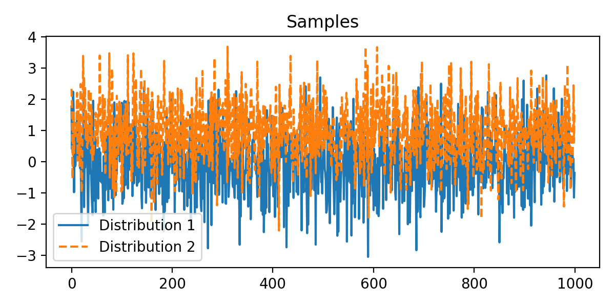
To gain a practical understanding of how these distance metrics behave, we can generate samples from two-dimensional Gaussian distributions and compute these distances as we vary the parameters of the distributions:

import numpy as np
import matplotlib.pyplot as plt
from scipy.stats import entropy
from scipy.stats import wasserstein_distance
from sklearn.neighbors import KernelDensity

# generate two uniform, random sample sets, with adjustable mean and std:
mean1, std1 = 0, 1  # Distribution 1 parameters (mean and standard deviation)
mean2, std2 = 1, 1  # Distribution 2 parameters (mean and standard deviation)
n = 1000
np.random.seed(0)  # Set random seed for reproducibility
sample1 = np.random.normal(mean1, std1, n)
np.random.seed(10)  # Set random seed for reproducibility
sample2 = np.random.normal(mean2, std2, n)

# plot the two samples:
plt.figure(figsize=(6,3))
plt.plot(sample1, label='Distribution 1', lw=1.5)
plt.plot(sample2, label='Distribution 2', linestyle="--", lw=1.5)
plt.title('Samples')
plt.legend()
plt.show()

The two samples sets.

Thw tow samples sets, generated with different random seeds, are not 100% identical, but quite similar. To calculate the distances, we need to estimate the probability distributions from the samples. One way to do this is by using kernel density estimation (KDE):

# calculate KDE for the samples:
x = np.linspace(-5, 7, 1000)  # X values for KDE
kde_sample1 = KernelDensity(kernel='gaussian', bandwidth=0.2).fit(sample1[:, None])
pdf_sample1 = np.exp(kde_sample1.score_samples(x[:, None]))

kde_sample2 = KernelDensity(kernel='gaussian', bandwidth=0.2).fit(sample2[:, None])
pdf_sample2 = np.exp(kde_sample2.score_samples(x[:, None]))

# we normalize the distributions to make sure they sum to 1:
pdf_sample1 /= np.sum(pdf_sample1)
pdf_sample2 /= np.sum(pdf_sample2)

# plot the distributions:
plt.figure(figsize=(6,3))
plt.plot(pdf_sample1, label='Distribution 1', lw=2.5)
plt.plot(pdf_sample2, label='Distribution 2', linestyle="--", lw=2.5)
plt.title('Probability Distributions')
plt.legend()
plt.show()

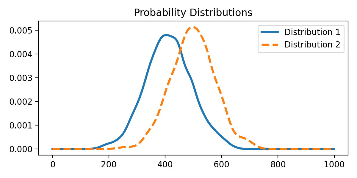The according probability distributions.

Now, we can compute the distances between the distributions:

# calculate the Wasserstein distance:
wasserstein_dist = wasserstein_distance(x, x, pdf_sample1, pdf_sample2)
print(f"Wasserstein Distance: {wasserstein_dist}")

# calculate the KL divergence between the two distributions:
epsilon = 1e-12
kl_divergence = entropy(pdf_sample1+epsilon, pdf_sample2+epsilon)
print(f"KL Divergence: {kl_divergence}")

# calculate the average distribution M:
pdf_avg = 0.5 * (pdf_sample1 + pdf_sample2)

# calculate the Jensen-Shannon divergence:
kl_divergence_p_m = entropy(pdf_sample1, pdf_avg)
kl_divergence_q_m = entropy(pdf_sample2, pdf_avg)
js_divergence = 0.5 * (kl_divergence_p_m + kl_divergence_q_m)
print(f"Jensen-Shannon Divergence: {js_divergence}")

# calculate the Total Variation distance:
tv_distance = 0.5 * np.sum(np.abs(pdf_sample1 - pdf_sample2))
print(f"Total Variation Distance: {tv_distance}")

# calculate the Bhattacharyya distance:
bhattacharyya_coefficient = np.sum(np.sqrt(pdf_sample1 * pdf_sample2))
bhattacharyya_distance = -np.log(bhattacharyya_coefficient)
print(f"Bhattacharyya Distance: {bhattacharyya_distance}")

Wasserstein Distance: 1.0307000718747261
KL Divergence: 0.6004132992619513
Jensen-Shannon Divergence: 0.12323025153055375
Total Variation Distance: 0.41218145262070593
Bhattacharyya Distance: 0.14151124108902025

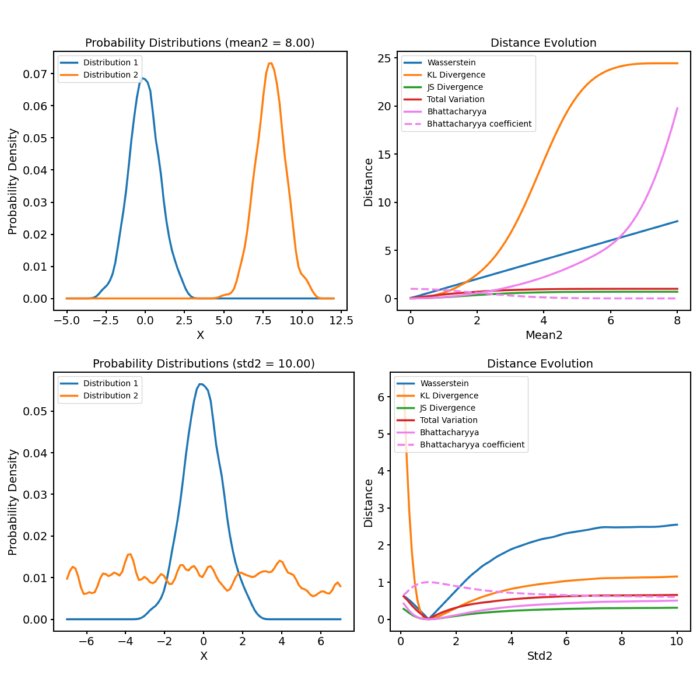
To get a better impression of how these metrics behave, we can plot them as a function of the parameters of the distributions. Let’s begin by varying the mean of one of the distributions:

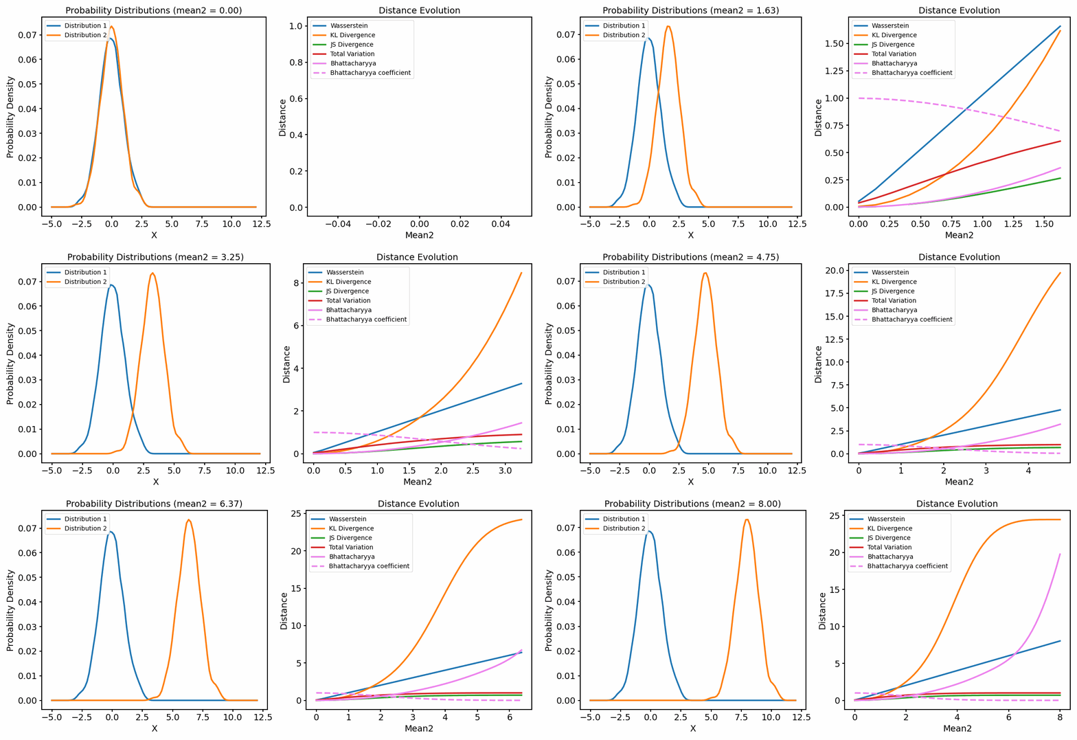The distance metrics (right panel) as a function of varying mean of one of the distributions (left panel). You can find the code for generating the animation in the GitHub repository mentioned below.

As we shift the two distributions apart from each other, all metrics behave differently:

The Wasserstein distance increases almost linearly within the calculated range, i.e., it responds with a constant increase to the shift of the two almost identical distributions.

The KL Divergence increases more rapidly, indicating a higher sensitivity to the shift. As long as the second distribution shifts apart from the first, but still overlaps with it, the KL Divergence shows s steep increase. However, once the second distribution moves beyond the first, the KL Divergence would become infinite due to the logarithm. However, we added a small $\epsilon\ll 1$ to prevent this from happening, so that we have further values which we can plot.

Both the JS Diversity and the TV Distance increase more slowly and converge to 1, indicating that the two probability distributions are becoming more and more dissimilar as their means diverge.

The Bahattacharyya coefficient starts with a value of 1, indicating that the two distributions are identical. This is not surprising, as at the beginning, the means of both distributions are equal. As the second distribution moves away from the first, the coefficient decreases until it converges to a value close to 0, indicating that the two distributions are completely dissimilar. Accordingly, the Bahattacharyya distance begins with a value of 0 and starts to increase more rapidly as the two distributions move further apart from each other.

Now, let’s have a look at how the metrics behave when we vary the standard deviation of one of the distributions:

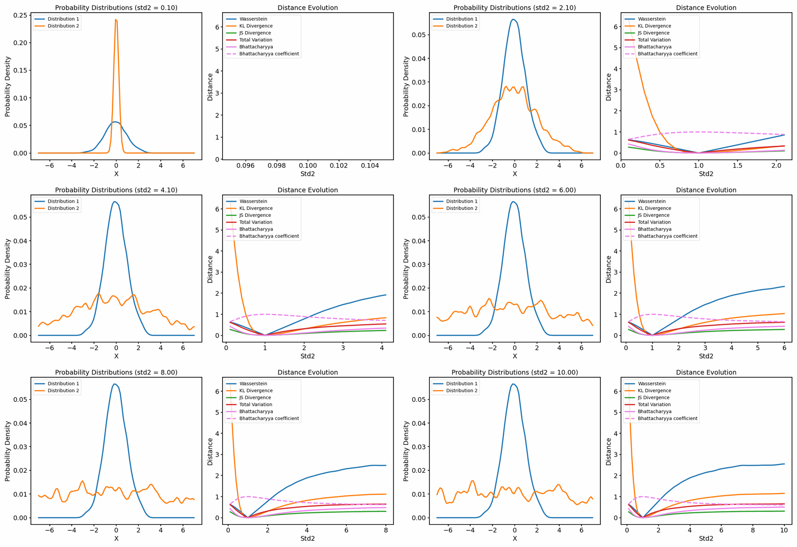The distance metrics (right panel) as a function of varying standard deviation of one of the distributions (left panel).

Let’s focus on what happens when the standard deviation of the second distribution is larger than one. Again, the metrics show increasing, but different behaviors:

The Wasserstein distance increases the fastest, indicating that it is the most sensitive to the change in the standard deviation, followed by the KL Divergence. Both show that the dissimilarity between the distributions increase as the standard deviation increases.

Both the JS Diversity and the TV Distance increase more slowly. However, this time, they converge to a much lower value than 1, indicating a dissimilarity between the distributions, but not as strong as in the previous case.

Also the Bahattacharyya diverges more slowly and converges to a value $\ll 1$, also indicating that the two distributions are dissimilar, but not as much as in the previous case.

Conclusion

Each of these metrics responds differently to shifts and variances in the probability distributions, revealing their unique sensitivities and properties. The Wasserstein distance, characterized by a nearly linear increase in response to distributional shifts, shows its particular strength in identifying structural changes in the underlying distributions. This feature makes it favored when working with generative models (e.g., GANs), where the positioning of the distributions in the feature space is crucial.

The KL Divergence, with its steep increase followed by a plateau (avoiding infinity due to a small $\epsilon$ addition), reflects its sensitivity towards divergences and its potential for capturing information loss when one distribution is used to represent another. Its propensity for rapid growth makes it ideal for applications where sensitivity to divergence is vital, such as in Variational Autoencoders (VAEs).

The JS Divergence and TV Distance, converging to a value of 1 as distributions diverge, provide a more tempered and normalized measure of dissimilarity. Their slower increase suggests that these metrics are less sensitive to extreme changes, making them appropriate for scenarios that require stable measurements, such as text classification or natural language processing.

Finally, the Bhattacharyya Distance and coefficient offer a unique perspective by measuring the overlap between two statistical samples. As distribution parameters diverge, the coefficient decreases (and distance increases) at a faster pace, making it robust and valuable in tasks requiring decisive binary decisions, such as pattern recognition tasks.

Notably, all metrics show distinct responses to changes in standard deviation, reinforcing the notion that the choice of metric should be informed by the specificities of the data and the problem at hand. The Wasserstein Distance and KL Divergence proved to be the most responsive to changes in standard deviation, while the JS Divergence, TV Distance, and Bhattacharyya Distance showed slower convergence and less sensitivity to such changes.

To conclude, the appropriate choice of a probabilistic distance metric depends not just on the theoretical properties of these metrics, but more importantly on the practical implications of these properties in the context of the specific machine learning task at hand. From comparing the performance of different models, assessing the similarity of different clusters, to testing statistical hypotheses, these metrics provide a mathematical backbone that supports machine learning. Rigorous examination and understanding of these metrics’ behavior under different conditions is a key aspect of their effective utilization.

The code used in this post is available in this GitHub repositoryꜛ.

If you have any questions or suggestions, feel free to leave a comment below or reach out to me on Mastodonꜛ.