Comparing Wasserstein distance, sliced Wasserstein distance, and L2 norm

In machine learning, especially when dealing with probability distributions or deep generative models, different metrics are used to quantify the ‘distance’ between two distributions. Among these, the Wasserstein distance, sliced Wasserstein distance, and the L2 norm, play an important role. In this blog post, we compare these metrics and discuss their advantages and disadvantages.

Wasserstein distance

We discussed the Wasserstein distance and its mathematical foundation already on some of my recent posts. To recap, the Wasserstein distance is a measure of the distance between two probability distributions that takes the geometry of the data space into account. The distance is computed by finding the optimal transport plan that transforms one distribution into the other with the minimum overall cost. The $p$-Wasserstein distance between two probability distributions $P$ and $Q$ defined on a metric space $(X, d)$ is defined as follows:

\[W_p(P, Q) = \left( \inf_{\gamma \in \Gamma(P,Q)} \int_{X \times X} d(x,y)^p d\gamma(x,y) \right)^{1/p}\]

where $\Gamma(P,Q)$ is the set of all couplings of $P$ and $Q$, and $d(x,y)$ is the distance between $x$ and $y$ in $X$. $p$ controls the order of the distance metric, with $p=1$ being the 1-Wasserstein distance, $p=2$ the 2-Wasserstein distance, and so on. The 1-Wasserstein distance is also known as the Earth Mover’s distance (EMD), since it can be interpreted as the minimum amount of ‘work’ required to transform one distribution into the other.

The Wasserstein distance provides a powerful and flexible distance measure between distributions. However, it is computationally demanding to calculate, especially for high-dimensional data. See, for example, the discussion in the post on the Sinkhorn algorithm.

Sliced Wasserstein distance

To mitigate the computational difficulties associated with the Wasserstein distance, the Sliced Wasserstein Distance (SWD) was introduced. This method uses the simple idea of transforming a complex high-dimensional problem into a collection of easier 1-dimensional problems.

The SWD between two probability distributions $P$ and $Q$ in $\mathbb{R}^d$ is defined as follows:

\[SWD(P, Q) = \int_{S^{d-1}} W_1(P_\theta, Q_\theta) d\theta\]

where $S^{d-1}$ is the unit sphere in $\mathbb{R}^d$, $P_\theta$ and $Q_\theta$ are the 1D distributions of $P$ and $Q$ projected onto the direction $\theta$, and $W_1$ is the 1-Wasserstein distance. Essentially, the SWD slices the distributions into multiple 1D distributions and computes the 1-Wasserstein distance for each slice, then averages these distances.

Although the SWD is an approximation of the true Wasserstein distance, it’s more computationally efficient and has been found to be useful in practice, particularly for training generative models.

L2 norm

The L2 norm, also known as the Euclidean distance, is a standard measure of distance between two points in a Euclidean space. Given two vectors $x$ and $y$ in $\mathbb{R}^d$, the L2 norm is defined as:

\[\|x - y\|_2 = \sqrt{\sum_{i=1}^d (x_i - y_i)^2}\]

While the L2 norm is simpler and faster to compute than the Wasserstein or sliced Wasserstein distances, it doesn’t take into account the geometry of the data space, and so it may not accurately represent the distance between or dissimilarity of two distributions.

Comparative analysis

To gain a practical understanding of how these distance metrics behave, we can generate samples from two-dimensional Gaussian distributions and compute these distances as we vary the parameters of the distributions.

Let’s first create two identical 2D Gaussian sample sets:

import numpy as np
import matplotlib.pyplot as plt
import matplotlib.animation as animation
from scipy.linalg import norm
import ot

# generate two 2D gaussian samples sets:
n = 50  # nb samples
m1  = np.array([0, 0])
m2  = np.array([4, 4])
s_1 = 1
s_2 = 1
cov1 = np.array([[s_1, 0], [0, s_1]])
cov2 = np.array([[s_2, 0], [0, s_2]])
np.random.seed(0)
xs = ot.datasets.make_2D_samples_gauss(n, m1, cov1)
np.random.seed(0)
xt = ot.datasets.make_2D_samples_gauss(n, m2, cov2)

# plot the distributions:
fig = plt.figure(figsize=(5, 5))
plt.plot(xs[:, 0], xs[:, 1], '+', label=f'Source (random normal,\n $\mu$={m1}, $\sigma$={s_1})')
plt.plot(xt[:, 0], xt[:, 1], 'x', label=f'Target (random normal,\n $\mu$={m2}, $\sigma$={s_2})')
plt.legend(loc=0, fontsize=10)
plt.xlabel('x')
plt.ylabel('y')
plt.axis('equal')
plt.xlim(-10, 10)
plt.ylim(-10, 10)
plt.title(f'Source and target distributions')
plt.tight_layout()
plt.show()

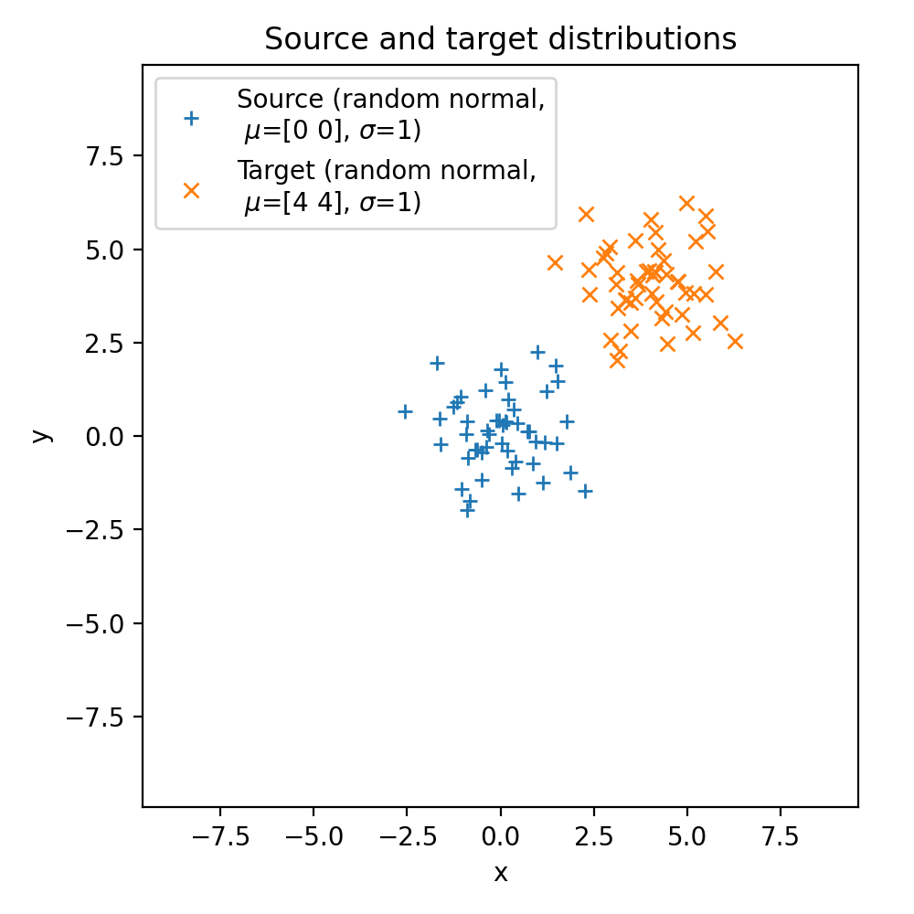The two Gaussian samples sets. The two samples are identical (np.random.seed() is reset to zero when generating the samples), but the means and standard deviations are adjustable, so we can vary them to see how the metrics change.

The means and standard deviations are adjustable, so we can vary them to see how the distances change.

Next, we calculate the standard Wasserstein distance between the two samples using the Python Optimal Transport (POT) libraryꜛ, which is based on linear programming:

# loss matrix:
M = np.sum((xs[:, np.newaxis, :] - xt[np.newaxis, :, :]) ** 2, axis=-1)
M /= M.max()

# transport plan:
G0 = ot.emd(a, b, M)

# Wasserstein distance:
w_dist = np.sum(G0 * M)

The sliced Wasserstein distance is calculated by first projecting the samples onto a random direction and then computing the 1-Wasserstein distance between the projected samples. We use the ot.sliced_wasserstein_distance function from the POT library, where this calculation is already implemented:

# sliced Wasserstein distance:
n_projections=1000
a, b = np.ones((n,)) / n, np.ones((n,)) / n  # uniform distribution on samples
w_dist_sliced = ot.sliced_wasserstein_distance(xs, xt, a, b, n_projections, seed=0)
wasserstein_distances_sliced.append(w_dist_sliced)

a and b represent discrete probability distributions of the source and target, respectively. Both are required when using the POT library. In our case, a and b are uniform distributions, meaning each sample point in the source and target distributions are equally likely. We use uniform distributions because we are dealing with sets of samples where there is no reason to believe any sample is more likely than any other. We assume no additional information about the distribution of the samples. In any other case, where the sample points are not equally likely, a and b would be different and not uniform. These cases might occur, for example, when dealing with weighted samples from some underlying distribution.

Lastly, we calculate the L2 norm between the two samples:

# calculate the L2 distance:
L2_dist = np.sqrt(norm(xs - xt))
l2_distances.append(L2_dist)

To demonstrate how the distances change as we, e.g., vary the means, let’s compute the three metrics for three different sets of means and standard deviations and plot the according distributions:

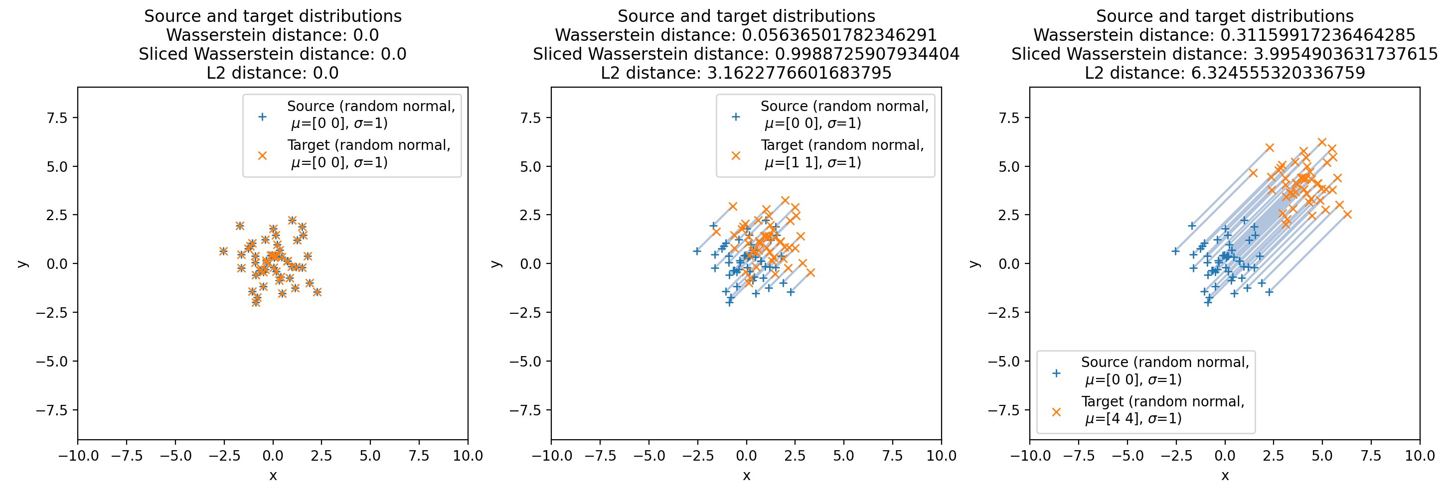The target set is shifted apart from the source set by 0 (left), 1 (middle) and 4 (right) units in both the x and y directions. The according distances, shown in the title of the plots, increase as the distance between the two sets increases.

As we can see, the metrics increase as the distance between the two sets increases. However, the speed of increase of the metrics differ among each other. The L2 norm increases the fastest, followed by the sliced Wasserstein distance, and the Wasserstein distance increases the slowest. To get a more comprehensive impression of how the metrics change as we vary the means and standard deviations, we can repeat the above procedure, but now for a range of means and standard deviations. The following plots are a saved animation of the results (you can find the full animation code in the GitHub repository mentioned below):

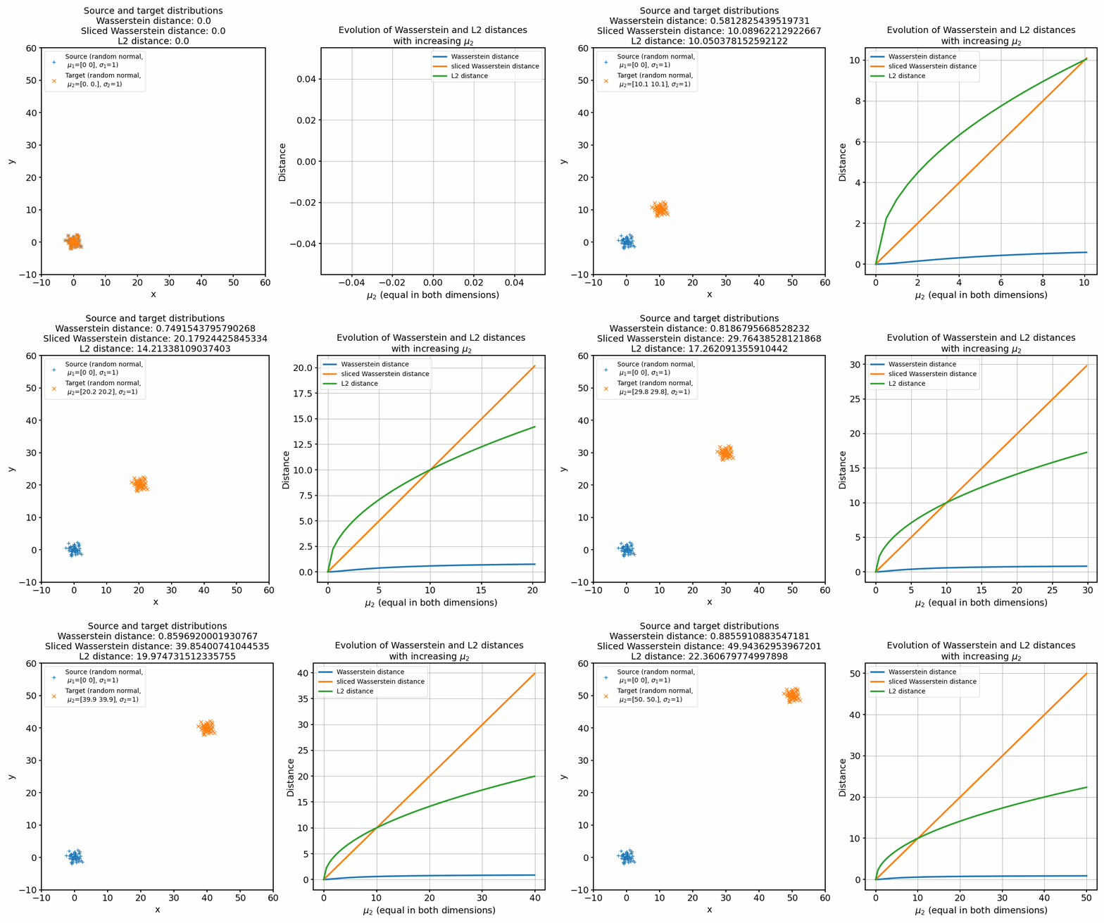Animation of continuously shifting the target distribution apart from the source distribution (left panel) and the according distances (right panel).

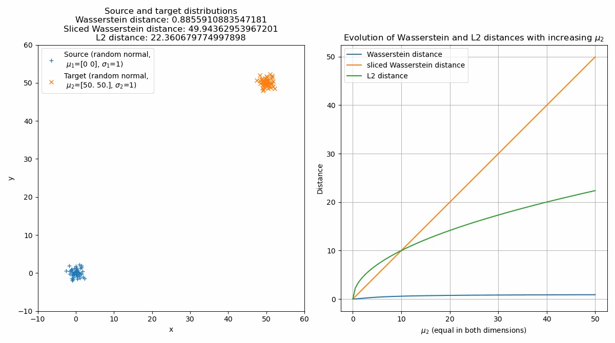
Seeing the behavior of the metrics now on a broader range, we can observe that indeed all metrics evolve differently for increasing means of the target set.

The default Wasserstein distance shows the least steep increase and slowly converges to $\sim$1, while the slices Wasserstein distance increases almost linearly. The reason for this lies in the differences in how the Wasserstein distance and the sliced Wasserstein distance are computed. For the Wasserstein distance, if we shift one identical distribution along any axis by a constant value, the cost of moving each “pile of earth” from the source distribution to the corresponding “hole” in the target distribution stays the same, because the mass it needs to be moved stays constant, regardless of how much the distribution is shifted. Since we normalize the cost matrix (M /= M.max()), which we do for reasons of numerical stability, also the distance stays the same (the maximum pairwise distance is 1). The sliced Wasserstein distance, on the other hand, is computed by projecting the distributions onto random lines and computing the Wasserstein distance between these one-dimensional projections. When we shift the distributions apart, these one-dimensional Wasserstein distances will tend to increase, leading to an increase in the overall SWD. The SWD, therefore, can capture absolute location differences more sensitively, whereas the standard Wasserstein distance is more focused on shape differences. This also applies to the increase of the standard deviation of the target distribution while keeping the means fixed, as we can see in the following animation:

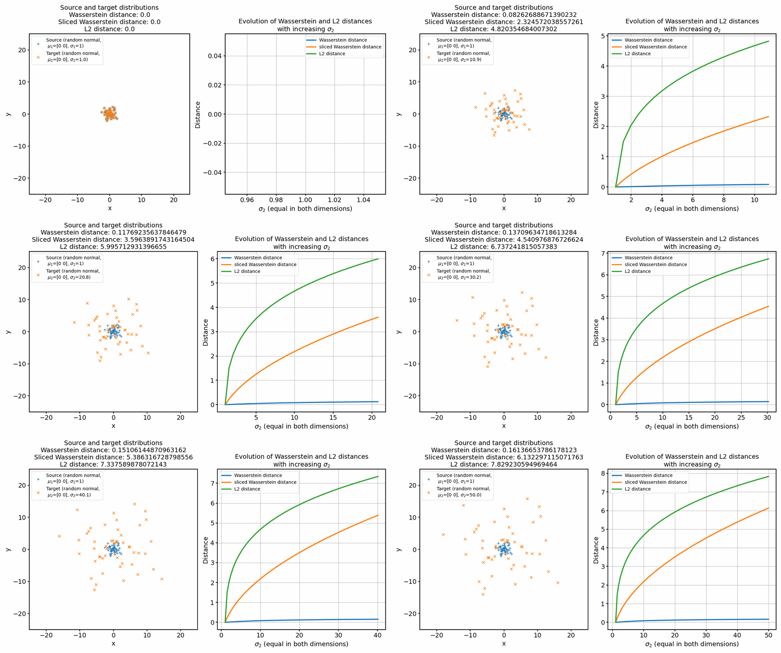Animation of continuously increasing the standard deviation of the target distribution.

The explanation for the observable behavior of the Wasserstein distance and the sliced Wasserstein distance are still the same. The increase of the standard deviation affects the spread and dispersion of the data points. But, as the global structure and mass of the distributions remain the same, the optimal transport plan will again not change, leading to only a small increase of the Wasserstein distance. The sliced Wasserstein distance, on the other hand, will increase more strongly, as the one-dimensional Wasserstein distances will increase with increasing standard deviation.

The L2 norm, on the other hand, increases the fastest, as it is not concerned with the shape of the distributions, but only with the distance between the points. However, when only shifting the target distribution apart from the source distribution, this holds true only until a certain distance, after which the SWD becomes the fastest. The L2 norm measures the straight-line distance between two points in a Euclidean space. When two distributions are close to each other, small changes in their locations or shapes can result in noticeable changes in the L2 distance. Therefore, in the early stages of the animation, as the mean of the target distribution starts to move away from the source distribution, the L2 norm increases rapidly. However, as the target distribution continues to move further away from the source distribution, the L2 norm’s rate of increase tends to slow down. This is because the L2 norm is essentially measuring the straight-line distance from the source to the target, which becomes less sensitive to changes when the two distributions are already far apart.

On the other hand, the sliced Wasserstein distance considers the optimal transportation cost of transforming one distribution into another, not just the straight-line distance between their means. In the early stages, when the two distributions are close to each other, the optimal transport plan can be relatively simple and inexpensive, leading to a smaller SWD. As the target distribution continues to move away from the source, the transportation cost increases, and hence the SWD increases. However, since SWD considers the entire structure of the distributions, not just their means, it can be more sensitive to changes when the distributions are far apart. This can lead to a faster increase in SWD compared to the L2 norm in the later stages of the animation.

Conclusion

Our examination of the Wasserstein distance, sliced Wasserstein distance (SWD), and L2 norm reveal fundamental differences in how these metrics capture variations between distributions. Each metric’s behavior under changing parameters of the distributions provides valuable insight into their optimal applications in machine learning tasks:

• The Wasserstein distance, characterized by its insensitivity to translation and focus on shape differences, is best suited to tasks where the overall shape of the distribution is paramount, such as in generative models like Generative Adversarial Networks (GANs) . It provides a more robust comparison by considering the minimal cost of transforming one distribution into another, ignoring simple translations.

• The sliced Wasserstein distance, with its sensitivity to both location and dispersion changes, can be more beneficial in tasks requiring an understanding of both shape and location changes. For instance, in outlier detection or tasks that demand a nuanced understanding of how distributions can vary.

• The L2 norm, due to its high sensitivity to point-to-point distances, is often most applicable in tasks like regression or clustering, where Euclidean distances between data points are of primary interest.

In conclusion, choosing the correct distance metric should be based on the specific requirements of the underlying task, considering the importance of shape, location, dispersion, and point-to-point distances in the data.

The code used in this post is available in this GitHub repositoryꜛ.

If you have any questions or suggestions, feel free to leave a comment below.