Understanding entropy

In physics, entropy is a fundamental concept that plays a crucial role in understanding the behavior of physical systems. It provides a measure of the disorder or randomness within a system, and its study has far-reaching applications across various branches of physics. This blog post aims to provide a brief overview of entropy in order to gain a better understanding of it.

What is entropy?

Imagine you have a box filled with gas molecules. The molecules are bouncing around, colliding with each other and the walls of the box. The more disordered or random the motion of these molecules, the higher the entropy of the gas.

Now imagine you have two boxes, one with hot gas and one with cold gas. If you connect the two boxes with a tube, heat will flow from the hot box to the cold box until both boxes are at the same temperature. This process increases the entropy of the system because heat flow increases disorder.

In general, natural processes tend to increase entropy. For example, when you drop an egg on the floor, it breaks and becomes more disordered. When you burn wood, the chemical bonds in the wood break and release energy, increasing disorder. When you mix cream into coffee, the cream spreads out and becomes more disordered. All of these processes increase entropy.

Mathematical description

Entropy is associated with statistical mechanics and thermodynamics. In statistical mechanics, the entropy of a system is closely related to the number of microscopic configurations that are consistent with the macroscopic properties of the system. In thermodynamics, entropy is linked to the second law, which states that the entropy of an isolated system tends to increase or remain constant over time. The mathematical representation of entropy depends on the context and the specific system under consideration. However, one common expression for entropy is given by Boltzmann’s entropy formula:

\[S = k \ln W\]

where $S$ represents the entropy, $k$ is the Boltzmann constant, and $W$ is the number of microscopic configurations or microstates corresponding to the macroscopic state of the system.

The change in entropy of a system can be determined via:

\[\Delta S = \int \frac{\delta Q}{T}\]

where $\Delta S$ represents the change in entropy, $\delta Q$ is the infinitesimal amount of heat transferred to or from the system, and $T$ is the temperature.

Entropy as function of microstates

To gain a better understanding of entropy, let’s demonstrate its calculation in Python. We will consider a simple example of a gas particle system. The microstates of the system are the different configurations or arrangements that the gas particles can take. The entropy of the system can be calculated using Boltzmann’s formula:

import numpy as np
import matplotlib.pyplot as plt
from scipy.stats import gaussian_kde

def calculate_entropy(microstates):
    entropy = np.log(microstates)
    return entropy

# Sample data of microstates
microstates = np.array([10, 20, 30, 15, 25])

# Calculate entropy using Boltzmann's formula
entropy = calculate_entropy(microstates)

# Display results
print("Entropy:", entropy)

# Plotting the entropy
plt.plot(range(len(microstates)), entropy)
plt.xlabel("System")
plt.ylabel("Entropy")
plt.title("Entropy of the Gas Particle System")
plt.show()

In the provided code, we define a function calculate_entropy that computes the entropy according Boltzmann’s formula. The sample data consists of the number of microstates corresponding to different configurations of a gas particle system. The plot demonstrates, that the entropy increases and decreases with the number of microstates:

• System $0$ with $N=10$,
• System $1$ with $N=20$,
• System $2$ with $N=30$,
• System $3$ with $N=15$, and
• System $4$ with $N=25$.

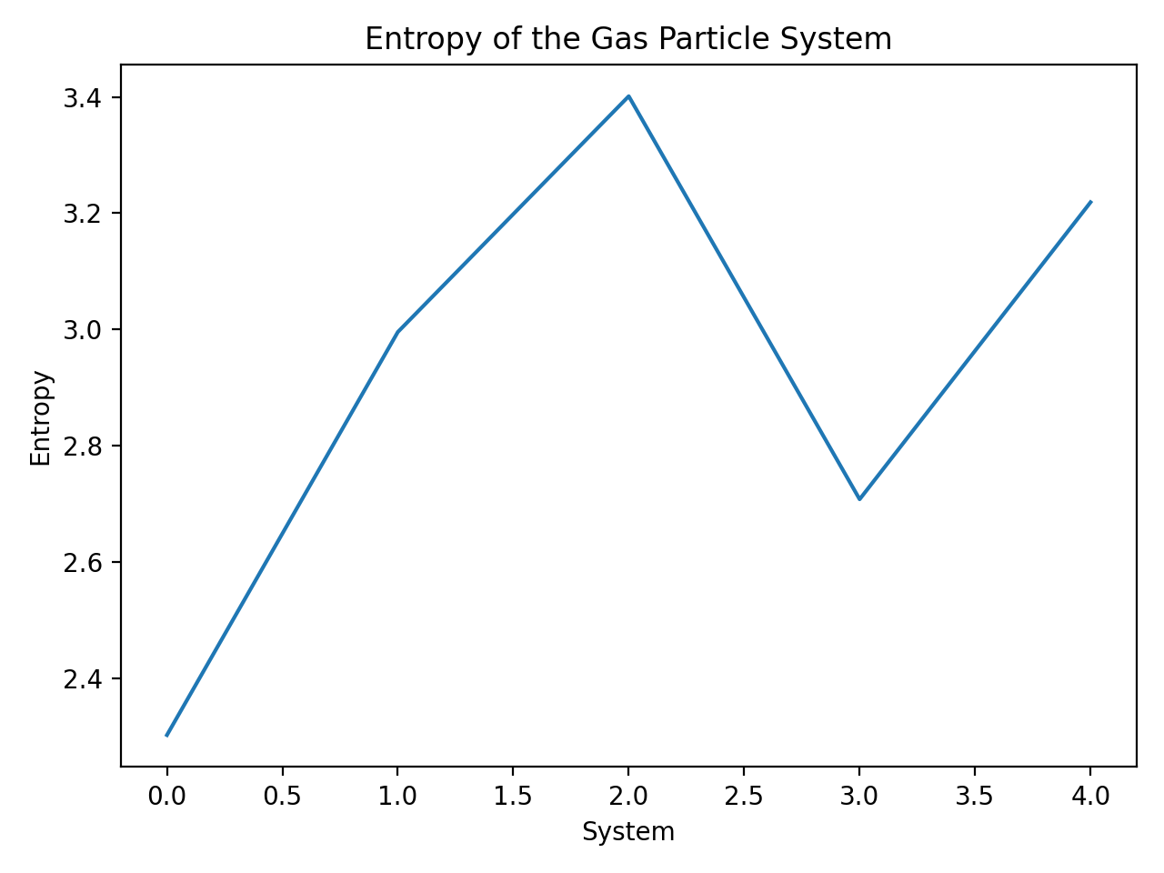The entropy of the gas particle system. The entropy changes with the number of microstates (here: System 0 with $N=10$, System 1 with $N=20$, System 2 with $N=30$, System 3 with $N=15$, System 4 with $N=25$).

Temporal evolution of entropy

Let’s consider another example. This time, we start with one microstate, that changes over time: after each time step, the number of microstates is increased by a random number between -2 and 3:

# set random seed for reproducibility
np.random.seed(41)

# Initialize the gas particle system
time_steps = 61  # 60 seconds + 1 (for indexing)
initial_microstates = 5
microstates = [initial_microstates]

# Simulate the evolution of the gas particle system
for t in range(1, time_steps):
    # Update the number of microstates based on a specific process
    if t <= 55:
        new_microstates = microstates[t-1] + np.random.randint(-2, 3)
    else:
        new_microstates = microstates[t-1] - 1  # Entropy decrease 5 seconds before the end
    microstates.append(new_microstates)

# Calculate entropy using Boltzmann's formula
entropy = calculate_entropy(microstates)

# Display results
print("Microstates:", microstates)
print("Entropy:", entropy)

# Plotting the entropy over time
time = np.arange(0, time_steps)  # Time in seconds
plt.plot(time, entropy)
plt.xlabel("Time (seconds)")
plt.ylabel("Entropy")
plt.title("Entropy of the Gas Particle System over Time")
plt.tight_layout()
plt.savefig("entropy_time.png", dpi=200)
plt.show()

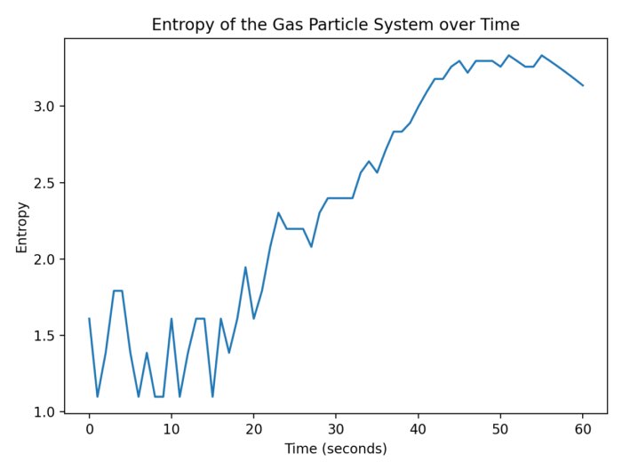
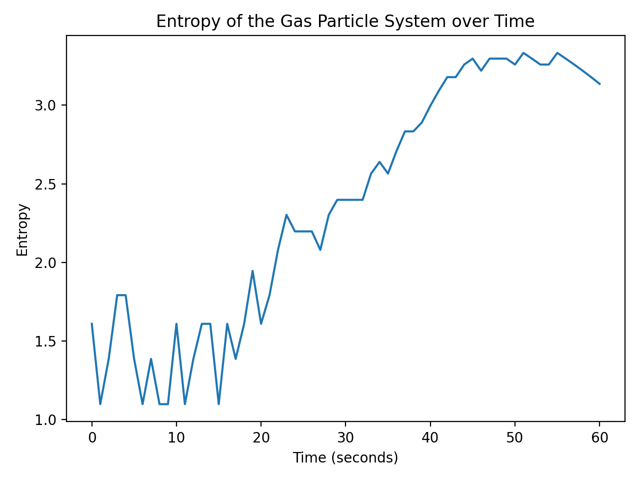The entropy of the gas particle system over time. The entropy increases over time since the number of microstates increases more or less steadily as a function of time.

In the given setup, the entropy increases over time since the number of microstates increases more or less steadily as a function of time.

Note, that the code allows the microstates to become zero, which causes negative logarithms in the entropy calculation. This is not a problem for the code and just a simplification for the sake of the example. However, this is not physically meaningful as it means, that the system evolved to a state where there are no possible configurations or microstates. I.e., it would imply that the system is in a highly ordered or singular state. A system with zero microstates would have perfect knowledge and predictability, resulting in no entropy. However, the presence of entropy is a fundamental aspect of physical systems. In a real system, the entropy would not decrease below a certain value, which is called the ground state. The defined random state np.random.seed(41) ensures non-zero microstates. Change this value to simulate different microstate and entropy evolutions.

Additionally, a specific process is introduced in the for loop. We set a condition (if t <= 55) to update the number of microstates randomly within a certain range. After 55 seconds (t > 55), we intentionally decrease the number of microstates by one at each time step, causing a decrease in entropy towards the end of the simulation. This reflects a scenario where the system undergoes a process that reduces its overall disorder or randomness.

Before we continue with the next example, let’s deepen our understanding of temporal variations in entropy. In the previous example, we observed an increase in entropy over time. This is because the number of microstates increased over time. However, this is not always the case. Let’s consider another example, where the number of microstates remains constant over time:

def calculate_entropy(particles):
    """Calculate the entropy of a system of particles."""
    # Calculate the histogram of particle positions
    hist, _ = np.histogram(particles, bins=10, range=(0, 1), density=True)
    # Calculate the probabilities
    probs = hist / hist.sum()
    # Calculate the entropy
    entropy = -np.sum(probs * np.log(probs + 1e-9))
    return entropy

# Set random seed for reproducibility
np.random.seed(42)
# Number of time steps
T = 100
# Number of particles
N_values = [10, 25, 200]
# Create figure
fig, ax = plt.subplots()

# Loop over number of particles
for N in N_values:
    # Initialize particle positions
    particles = np.random.uniform(size=N)
    # Initialize entropy array
    S = np.zeros(T)
    # Loop over time steps
    for t in range(T):
        # Update particle positions
        particles += 0.01 * np.random.randn(N)
        # Calculate entropy
        S[t] = calculate_entropy(particles)
    # Plot entropy vs time
    ax.plot(S, label=f'N={N}')

# Add legend and labels
ax.legend()
ax.set_xlabel('Time')
ax.set_ylabel('Entropy')
plt.tight_layout()
plt.savefig("entropy_different_number_particles.png", dpi=200)
plt.show()

The code above calculates the entropy of three different systems of gas particles. The system vary in the number of particles, namely for $N=10$, $25$, and $200$ particles, respectively.The particle positions are updated at each time step by adding a small random number. The entropy is calculated using the probability density of the particle positions. The plot below shows the entropy of the system over time. The entropy remains constant over time since the number of microstates remains constant. However, the temporal fluctuations in entropy are larger for the system with fewer particles, and lower for the system with more particles. This is because the probability density of the particle positions is more spread out for the system with fewer particles, resulting in a higher entropy:

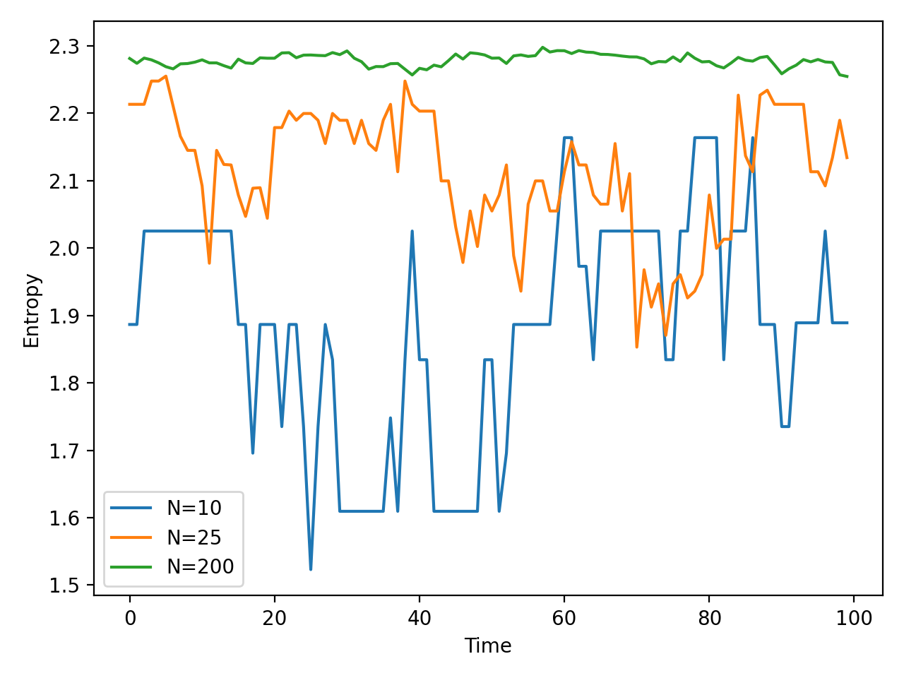The entropy of the gas particle system over time. The entropy remains constant over time since the number of microstates remains constant. However, the temporal fluctuations in entropy for each system.

Entropy of closed systems

If the previous example was a bit too abstract, let’s consider a more concrete example. We will now simulate the entropy of two closed systems. Both systems are filled with $N=10$ gas particles. The only difference between the two systems is the density of the gas particles. In the first system, the gas particles are densely packed, while in the second system, the gas particles are more spread out. Here is the corresponding code:

# re-defining the entropy function:
def entropy(probs):
    return -np.sum(probs * np.log(probs))

# Set random seed for reproducibility
np.random.seed(42)

# Number of particles
n = 10

# Generate particle positions for first box
x1 = np.random.normal(loc=0.5, scale=0.1, size=n)
y1 = np.random.normal(loc=0.5, scale=0.1, size=n)

# Generate particle positions for second box
x2 = np.random.uniform(size=n)
y2 = np.random.uniform(size=n)

# Calculate probability density for first box
kde1 = gaussian_kde(np.vstack([x1, y1]))
xgrid, ygrid = np.mgrid[0:1:100j, 0:1:100j]
probs1 = kde1(np.vstack([xgrid.ravel(), ygrid.ravel()]))
probs1 /= probs1.sum()

# Calculate probability density for second box
kde2 = gaussian_kde(np.vstack([x2, y2]))
probs2 = kde2(np.vstack([xgrid.ravel(), ygrid.ravel()]))
probs2 /= probs2.sum()

# Calculate entropy for each box
entropy1 = entropy(probs1)
entropy2 = entropy(probs2)

# Create figure and axes
fig, (ax1, ax2) = plt.subplots(ncols=2)

# Plot particle positions and probability density for first box
ax1.scatter(x1, y1)
im1 = ax1.imshow(np.fliplr(probs1.reshape(xgrid.shape)), origin='upper', extent=[0, 1, 0, 1])
ax1.set_title(f'System 1: Entropy = {entropy1:.3f}')
cbar1 = plt.colorbar(im1, ax=ax1, orientation='horizontal', label='Probability Density')
cbar1.ax.set_xticklabels(cbar1.ax.get_xticklabels(), rotation=90)
ticks = np.linspace(im1.get_clim()[0], im1.get_clim()[1], 4)
cbar1.set_ticks(ticks)

# Plot particle positions and probability density for second box
ax2.scatter(x2, y2)
im2 = ax2.imshow(np.fliplr(probs2.reshape(xgrid.shape)), origin='upper', extent=[0, 1, 0, 1])
ax2.set_title(f'System 2: Entropy = {entropy2:.3f}')
cbar2 = plt.colorbar(im2, ax=ax2, orientation='horizontal', label='Probability Density')
cbar2.ax.set_xticklabels(cbar2.ax.get_xticklabels(), rotation=90)
ticks = np.linspace(im2.get_clim()[0], im2.get_clim()[1], 4)
cbar2.set_ticks(ticks)
plt.tight_layout()
plt.savefig("entropy_two_systems.png", dpi=200)
plt.show()

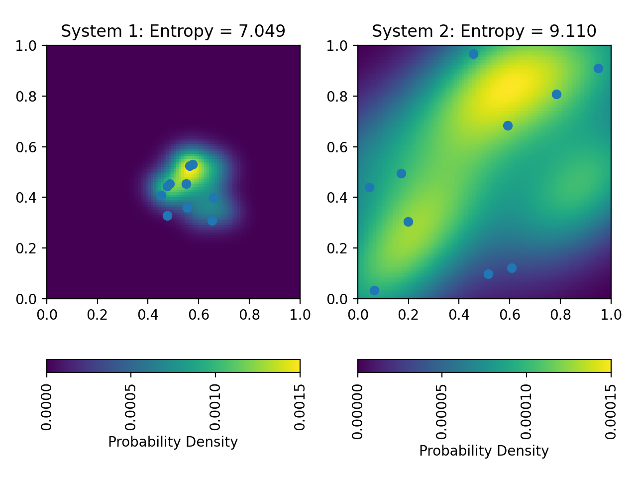The entropy of the two different closed systems. Plotted are the particle positions together with their probability density calculated using kernel density estimation. The latter is used as the probability to calculate the entropy of each system. In system 1, the particles are more densely packed (=more “ordered”) than in system 2 (see text below for implementation). This results in a lower entropy for system 1.

This code generates the two systems using different probability distributions for the particle positions. For the first system, we use a normal distribution centered at $(0.5, 0.5)$ with a small standard deviation to generate densely placed particles. For the second box, we use a uniform distribution to generate more widely spread particles. We then use kernel density estimation to calculate the probability density of the particle positions in each system. This gives us a continuous probability distribution that we can use to calculate the entropy of each system. Both the particle positions and the probability density are plotted for each system. The entropy of system 1 is lower than the entropy of system 2. This is because the particles in system 1 are more densely packed, i.e., the system is more “ordered”.

Conclusion

Entropy is a fundamental concept in physics that provides insights into the behavior of physical systems. Whether in the context of statistical mechanics or thermodynamics, understanding entropy allows us to quantify the disorder, randomness, and the number of possible configurations within a system. Hopefully, this post has helped you gain a better understanding of entropy and its applications. If you have any questions or suggestions, feel free to leave a comment below or reach out to me on Mastodonꜛ.

The code used in this post is also available in this GitHub repositoryꜛ.