Approximating the Wasserstein distance with cumulative distribution functions
In the previous two posts, we’ve discussed the mathematical details of the Wasserstein distance, exploring its formal definition, its computation through linear programming and the Sinkhorn algorithm. In this post, we take a different approach by approximating the Wasserstein distance with cumulative distribution functions (CDF), providing a more intuitive understanding of the metric.
Mathematical description
Let’s recap: Given two 1D distributions $P$ and $Q$, the first Wasserstein distance is defined as:
\[W_1(P, Q) = \inf_{\gamma \in \Gamma} \sum_{i,j} \gamma_{i,j} \cdot c_{i,j}\]where $\Gamma$ is the set of all joint distributions $\gamma(x, y)$ whose marginals are respectively $P$ and $Q$, and $c_{i,j}$ is the cost function, typically the absolute difference between $i$ and $j$.
The approximation method presented here calculates the cumulative distribution function (CDF) of the two distributions and then computes the area between these two CDFs. This area can be interpreted as the total “work” done to transform one distribution into the other, which is the essence of the Wasserstein distance.
Given the CDFs $F_P$ and $F_Q$ of the two distributions $P$ and $Q$, the total work is calculated as:
\[\text{Total work} = \int |F_P(x) - F_Q(x)| dx\]This integral can be approximated by a sum over discrete $x$ values:
\[\text{Total work} \approx \sum_{i} |F_P(x_i) - F_Q(x_i)| \cdot \Delta x_i\]where $\Delta x_i = x_{i+1} - x_i$ is the distance between the $x$ values.
Python example
Let’s apply the method to two distributions using Python. First, we’ll generate two discrete normally distributed sample sets. For ease of illustration, the sets are randomly generated, but identical (for both sets, np.random.seed() is reset to zero). However, the target set is shifted by one unit against the source set:
import numpy as np
import matplotlib.pyplot as plt
from scipy.stats import cumfreq
from scipy.stats import wasserstein_distance
from scipy.stats import norm
from scipy.interpolate import interp1d
import ot

# generate two 1D gaussian samples:
n=1000
x=np.linspace(-10, 10, n)
m1 = 0
m2 = 1
s1 = 1
s2 = 1
np.random.seed(2)
dist1 = norm.rvs(loc=m1, scale=s1, size=n)
np.random.seed(2)
dist2 = norm.rvs(loc=m2, scale=s2, size=n)

# plot the distributions:
plt.figure(figsize=(7, 3))
plt.plot(x, dist1, label=f"source ($\mu$={m1}, $\sigma$={s1})", alpha=1.00)
plt.plot(x, dist2, label=f"target ($\mu$={m2}, $\sigma$={s2})", alpha=0.55)
plt.xlabel('x')
plt.ylabel('y')
plt.legend()
plt.tight_layout()
plt.show()
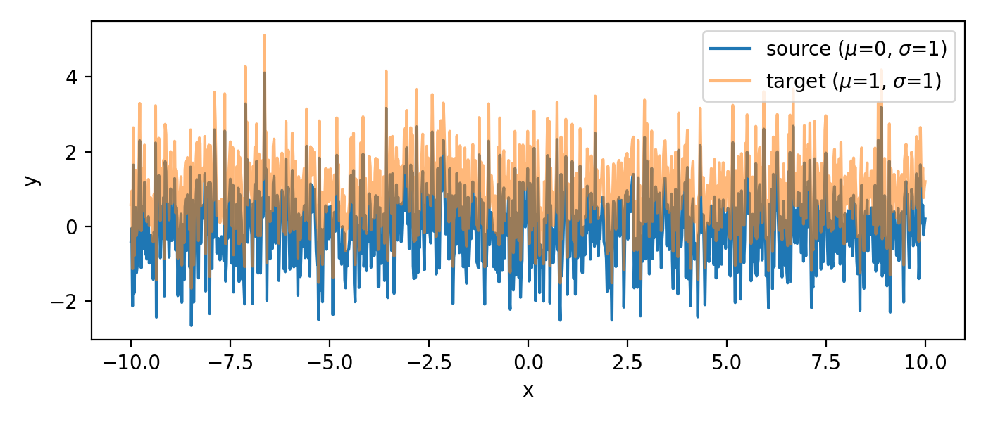 The two sample sets. Both are randomly generated, but identical. The target set is shifted by one unit ($\mu_2=1$) against the source set ($\mu_1=0$).
Next, we compute the CDFs of the two sets:
# compute the CDFs:
a = cumfreq(dist1, numbins=100)
b = cumfreq(dist2, numbins=100)

# compute the x-values for the CDFs:
x_a = a.lowerlimit + np.linspace(0, a.binsize*a.cumcount.size, a.cumcount.size)
x_b = b.lowerlimit + np.linspace(0, b.binsize*b.cumcount.size, b.cumcount.size)
We need to interpolate the CDFs to the same $x$ values to be able to calculate the area between them:
# interpolate the CDFs to the same x-values:
f_a = interp1d(x_a, a.cumcount / a.cumcount[-1])
f_b = interp1d(x_b, b.cumcount / b.cumcount[-1])
x_common = np.linspace(max(x_a[0], x_b[0]), min(x_a[-1], x_b[-1]), 1000)
cdf_a_common = f_a(x_common)
cdf_b_common = f_b(x_common)
To get an idea, how the underlying distributions look like, we can calculate and plot the probability density functions (PDFs) of the two distributions:
# calculate the PDF of the first distribution:
pdf_a = np.diff(cdf_a_common)
pdf_b = np.diff(cdf_b_common)

# plot the PDFs:
plt.figure(figsize=(7, 3))
plt.plot(pdf_a, label='source PDF')
plt.plot(pdf_b, label='target PDF')
plt.ylabel('probability density')
plt.legend()
plt.tight_layout()
plt.show()
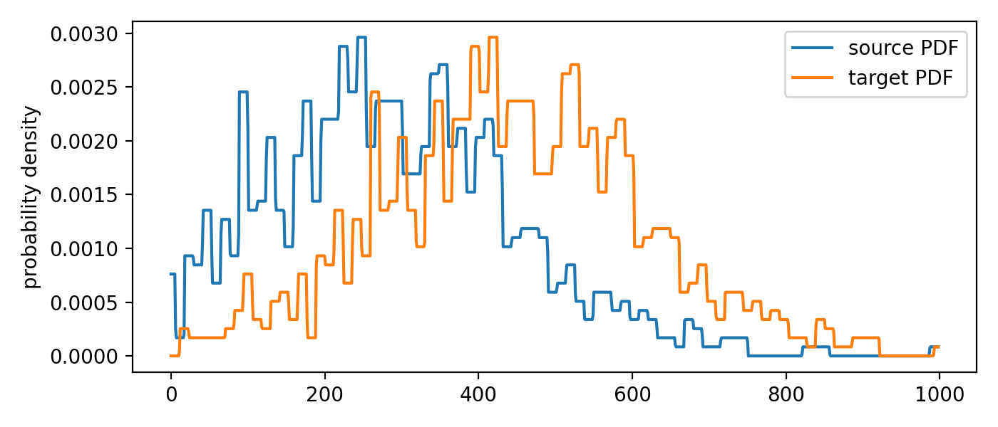 The according PDFs of the two distributions.
And the according CDFs:
# plot the CDFs:
plt.figure(figsize=(5.5, 5))
plt.plot(x_common, cdf_a_common, label='source CDF')
plt.plot(x_common, cdf_b_common, label='target CDF')
# plot the absolute difference between the CDFs:
plt.fill_between(x_common, cdf_a_common, cdf_b_common, color='gray', alpha=0.5, label='absolute difference')
plt.ylabel('cumulative frequency')
plt.legend()
plt.tight_layout()
plt.show()
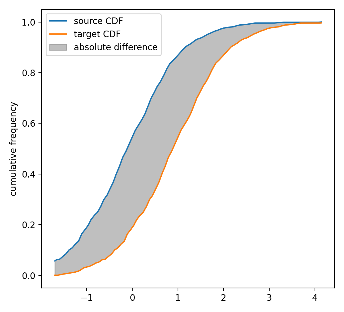 The CDFs of the two distributions. The grey shaded area indicates the absolute difference between the two CDFs, i.e., the “work” needed to transform the source into the target distribution. This “work” serves as an approximation of the Wasserstein distance.
The grey shaded area indicates the absolute difference between the two CDFs. It represents the total work needed to transform the source into the target distribution and serves as an approximation of the Wasserstein distance. To quantitatively assess the area, we first need to calculate the absolute difference between the two CDFs at each point and then multiply it by the distance between the points:
# compute the absolute difference between the CDFs at each point:
diff = np.abs(cdf_a_common - cdf_b_common)

# compute the distance between the points:
dx = np.diff(x_common)

# compute the total "work":
total_work = np.sum(diff[:-1] * dx)
print(f"Total work of the transport: {total_work}")
Total work of the transport: 0.9769786231313
For comparison, we calculate the Wasserstein distance using library functions:
print(f"Wasserstein distance (scipy): {wasserstein_distance(dist1, dist2)}")
print(f"Wasserstein distance W_1 (POT): {ot.wasserstein_1d(dist1, dist2, p=1)}")
Wasserstein distance (scipy): 1.0
Wasserstein distance W_1 (POT): 1.0000000000000007
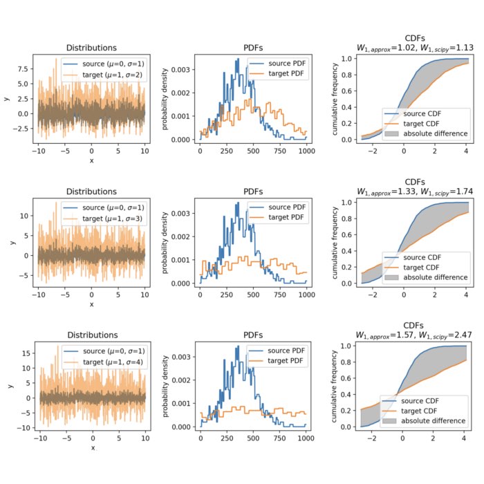
As you can see, the Wasserstein distance calculated with the approximation method is very close to the exact Wasserstein distance calculated with the scipy and POT library. However, keep in mind, that the two sample sets are identical and, though shifted, the dissimilarity between them is very low. If we increase the shift, the approximation becomes less accurate:


 Wasserstein approximation for differently shifted target distributions. The approximation becomes less accurate for increasing shifts (compared to the Wasserstein distance calculated with scipy).
The same accounts for increasing the variance of the target set:


 Wasserstein approximation for different standard deviations of the target set. Also here, the approximation becomes less accurate for increasing standard deviations (compared to the Wasserstein distance calculated with scipy).
In conclusion, the approximation can become less accurate for distributions with significant differences in their shapes or locations. However, the method is computationally efficient, especially for high-dimensional data, as it avoids the need for solving a linear programming problem. As long as the distributions are not too dissimilar, the approximation provides a valuable alternative for estimating the the Wasserstein distance. Another factor controlling the accuracy of the approximation is the granularity of the $x$ values. A finer grid will yield a more accurate approximation, but will also increase the computational cost.
Conclusion
The approximation of the Wasserstein distance by calculating the cumulative distribution function provides an intuitive and computationally efficient method to quantify the ‘distance’ between two distributions. While it may not always provide the exact Wasserstein distance, especially for dissimilar distributions, it offers a good estimate and I think it also helps to understand the underlying concept of the Wasserstein distance.
The code used in this post is available in this GitHub repositoryꜛ.
If you have any questions or suggestions, feel free to leave a comment below or reach out to me on Mastodonꜛ.
Comments
Comment on this post by publicly replying to this Mastodon post using a Mastodon or other ActivityPub/Fediverse account.
Comments on this website are based on a Mastodon-powered comment system. Learn more about it here.
There are no known comments, yet. Be the first to write a reply.