Decision Trees vs. Random Forests for classification and regression: A comparison
Decision trees and random forests are popular machine learning algorithms that are widely used for both classification and regression tasks. In this blog post, we elucidate their theoretical foundations and discuss the differences as well as their advantages and drawbacks.
 Image generated with DALL-E (sourceꜛ)
Decision trees
A decision tree is a flowchart-like structure where each internal node represents a test on a specific attribute, each branch represents the outcome of the test, and each leaf node represents a class label or a regression value. The decision-making process starts at the root node and follows a path down the tree until a leaf node is reached, providing the final prediction.
Mathematically, a decision tree can be defined as a function that maps an input vector, $x$, to an output value, $y$. Let’s denote the decision tree as $T$. For a given input vector, $T(x)$ provides the predicted output.
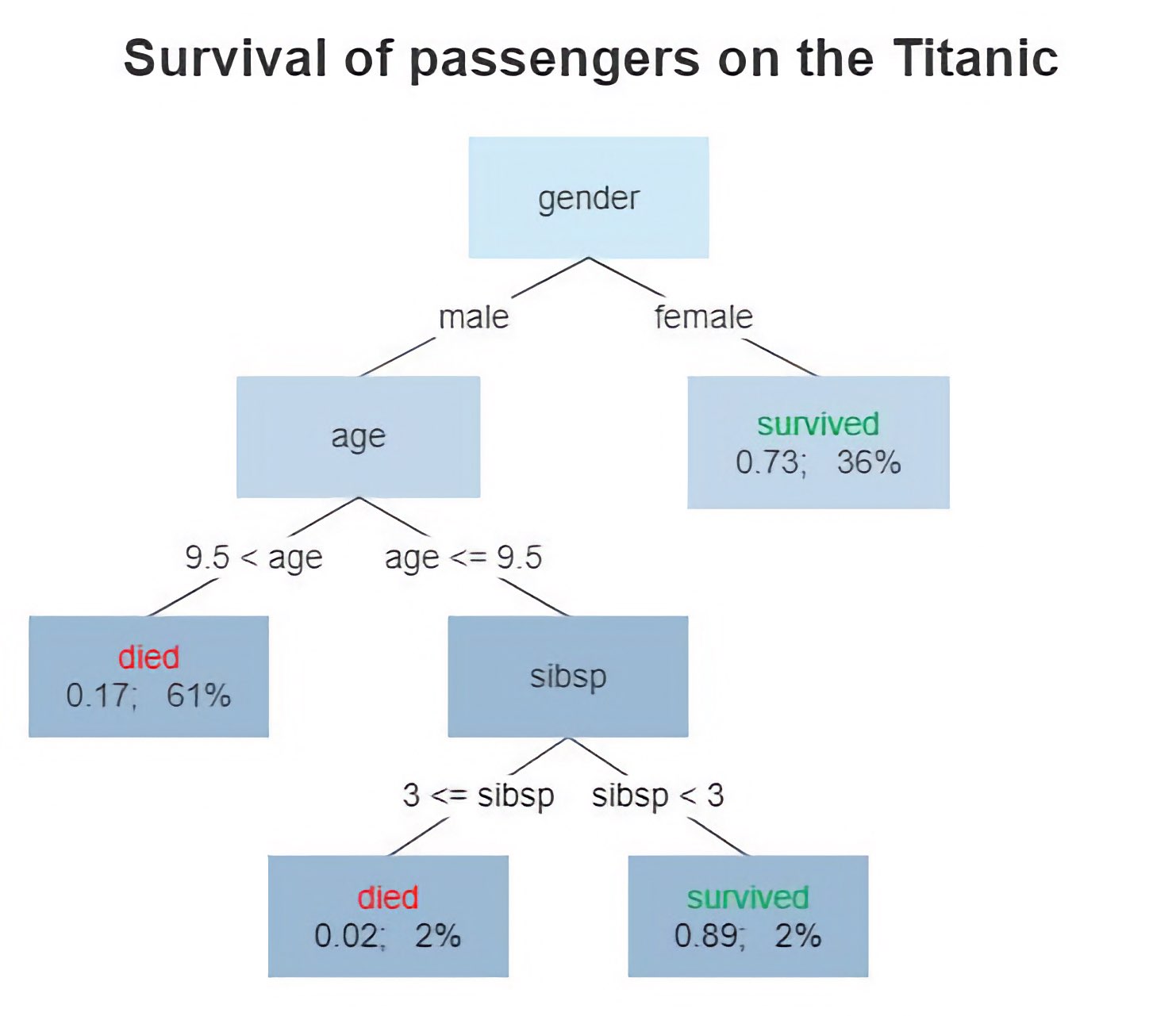 Diagram of a decision tree. The tree shows the survival of passengers on the Titanic. The figures under the leaves show the probability of survival and the percentage of observations in the leaf. “sibsp” is the number of spouses or siblings aboard. Source: Wikimediaꜛ (license: CC BY-SA 4.0)
Random forests
A random forest, on the other hand, is an ensemble learning method that combines multiple decision trees to make predictions. It creates an ensemble of decision trees and aggregates their predictions to make the final prediction. The fundamental idea behind random forests is to introduce randomness into the tree-building process.
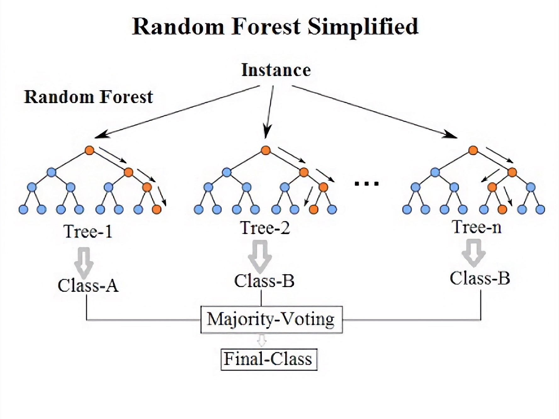 Diagram of a random decision forest. Source: Wikimediaꜛ (license: CC BY-SA 4.0)
The random forest algorithm involves two main steps: building the individual trees and combining their predictions. During the tree-building process, a random subset of features is selected at each split, and the best split is made based on a criterion such as information gain or Gini impurity (see box below). To make predictions, each tree in the random forest independently provides a prediction, and the final prediction is obtained by majority voting (for classification) or averaging (for regression) the individual tree predictions.
Gini impurity
Gini impurity is a measure of impurity or homogeneity used in decision tree algorithms for classification tasks. It quantifies the probability of incorrectly classifying a randomly chosen element in a dataset if it were randomly labeled according to the class distribution in that subset.
Mathematically, Gini impurity is defined as follows:
\[Gini(p) = 1 - \sum_{i=1}^{C} (p_i)^2\]where:
- $Gini(p)$ is the Gini impurity for a particular node or subset,
- $C$ is the number of classes,
- $p_i$ is the probability of an element belonging to class $i$.
The Gini impurity is calculated for each node in the decision tree during the tree construction process. The objective is to find the best splits that minimize the Gini impurity, resulting in pure or homogeneous subsets.
A Gini impurity of 0 indicates a perfectly pure node where all elements belong to the same class. Conversely, a Gini impurity of 1 indicates a node with equal probabilities for each class, implying maximum impurity or heterogeneity.
When constructing a decision tree, the algorithm evaluates different split points based on features and chooses the split that minimizes the weighted sum of Gini impurities for the resulting child nodes. The split that reduces the impurity the most is considered the best and is used to separate the data into different branches.
Thus, Gini impurity is a criterion used to assess the quality of splits and make decisions during the construction of decision trees. By minimizing the Gini impurity, the algorithm aims to create nodes that are as pure and homogeneous as possible, leading to accurate and meaningful classifications.
Differences and Advantages
Decision trees are relatively easy to interpret and visualize, as the decision-making process is represented in a hierarchical structure. In contrast, random forests are more complex and difficult to interpret due to the ensemble nature of the algorithm.
Decision trees are prone to overfitting, especially when the tree depth increases. Random forests mitigate this issue by aggregating predictions from multiple trees, which helps to reduce overfitting and improve generalization.
Decision trees are computationally efficient during training but can be slow during prediction, particularly for large trees. Random forests are faster during prediction, as they parallelize the process by leveraging multiple decision trees.
Random forests offer better robustness to noisy data and outliers compared to decision trees. The ensemble approach of random forests helps to minimize the impact of individual noisy or erroneous predictions.
Practical implementation in Python: Classification problem
Let’s demonstrate the implementation of decision trees and random forests using a classification problem in Python. We will use the famous Iris dataset for this example.
For reproducibility:
conda create -n random_forest_vs_decision_tree -y python=3.9
conda activate random_forest_vs_decision_tree
conda install -y mamba
mamba install -y scikit-learn matplotlib numpy ipykernel pandas scikit-image napari[all]
Here is the Python code:
# %% IMPORTS
from sklearn.datasets import load_iris, load_digits
from sklearn.model_selection import train_test_split
from sklearn.tree import DecisionTreeClassifier
from sklearn import tree
from sklearn.ensemble import RandomForestClassifier
import numpy as np
import matplotlib.pyplot as plt
from sklearn.datasets import fetch_california_housing
from sklearn.tree import DecisionTreeRegressor
from sklearn.ensemble import RandomForestRegressor
# %% MAIN
# load the Iris dataset:
data = load_iris()
X, y = data.data, data.target

# split the data into training and test sets:
X_train, X_test, y_train, y_test = train_test_split(X, y, test_size=0.2, random_state=42)

# decision tree classifier:
dt_classifier = DecisionTreeClassifier()
dt_classifier.fit(X_train, y_train)

# Visualizing the decision tree
plt.figure(figsize=(12, 8))
tree.plot_tree(dt_classifier, filled=True)
plt.show()


# random forest classifier:
rf_classifier = RandomForestClassifier(n_estimators=100)
rf_classifier.fit(X_train, y_train)

# get feature importances
importances = rf_classifier.feature_importances_
std = np.std([tree.feature_importances_ for tree in rf_classifier.estimators_], axis=0)
indices = np.argsort(importances)[::-1]

# convert feature names to a list:
feature_names = list(data.feature_names)

# plot feature importances:
plt.figure(figsize=(3, 4))
plt.bar(range(X.shape[1]), importances[indices], yerr=std[indices], align="center")
plt.xticks(range(X.shape[1]), [feature_names[i] for i in indices], rotation='vertical')
plt.xlabel('Features')
plt.ylabel('Importance')
plt.title('Feature Importance - Random Forest')
ax = plt.gca()
ax.spines['top'].set_visible(False)
ax.spines['right'].set_visible(False)
ax.spines['left'].set_visible(False)
ax.spines['bottom'].set_visible(False)
ax.xaxis.set_ticks_position('none')
plt.show()
Here is the trained decision tree:
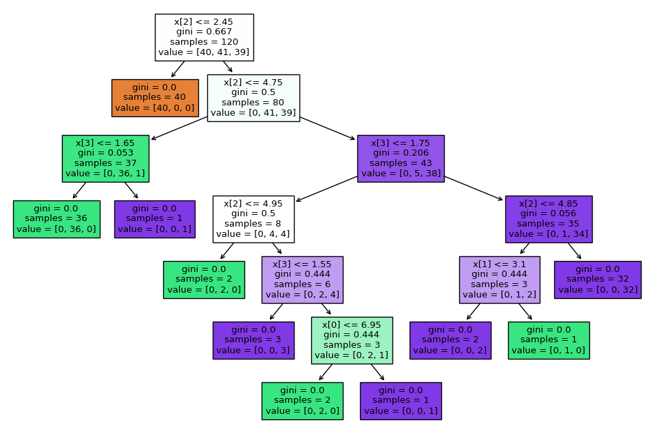 The decision tree trained on the Iris dataset.
Since a random forest consists of an ensemble collection of decision trees, its visual representation is somewhat more complex. Nevertheless, we can visualize the average importance of the features over alle decision trees in the Random Forest:
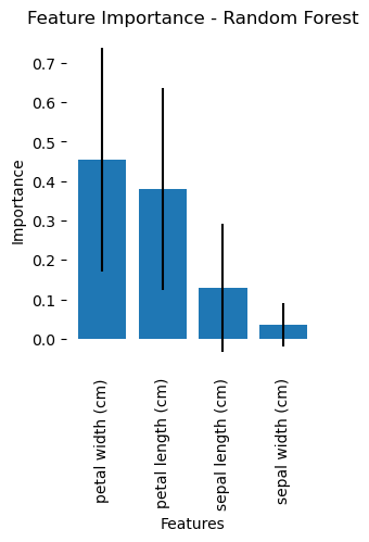 Average importance of the features over all decision trees in the random forest.
Practical implementation in Python: Regression problem
Decision trees and random forests can also be used for regression tasks. Let’s illustrate their implementation on a regression problem using the California Housing dataset.
# %% IMPORTS
from sklearn.datasets import fetch_california_housing
from sklearn.model_selection import train_test_split
from sklearn.tree import DecisionTreeRegressor
from sklearn.ensemble import RandomForestRegressor
from sklearn.metrics import r2_score, mean_squared_error
import numpy as np
import matplotlib.pyplot as plt
# %% REGRESSION PROBLEM

data = fetch_california_housing(as_frame=True)
X = data.data.loc[:, ['Longitude', 'Latitude', 'MedInc']]
y = data.target

# split the data into training and test sets
X_train, X_test, y_train, y_test = train_test_split(X, y, test_size=0.2, random_state=42)

# Decision tree regressor
dt_regressor = DecisionTreeRegressor()
dt_regressor.fit(X_train, y_train)

# random forest regressor
rf_regressor = RandomForestRegressor(n_estimators=100)
rf_regressor.fit(X_train, y_train)

# predict on the test set
dt_predictions = dt_regressor.predict(X_test)
rf_predictions = rf_regressor.predict(X_test)

# calculate metrics:
dt_r2 = r2_score(y_test, dt_predictions)
rf_r2 = r2_score(y_test, rf_predictions)
dt_mse = mean_squared_error(y_test, dt_predictions)
rf_mse = mean_squared_error(y_test, rf_predictions)

# plot predicted versus actual values
plt.figure(figsize=(10, 5))
plt.scatter(y_test, dt_predictions, color='b', label='Decision Tree' + f", R$^2$: {dt_r2:.3f}", alpha=0.4)
plt.scatter(y_test, rf_predictions, color='r', label='Random Forest' + f", R$^2$: {rf_r2:.3f}", alpha=0.4)
plt.plot([y_test.min(), y_test.max()], [y_test.min(), y_test.max()], 'k--', lw=2)
plt.xlabel('Actual Values')
plt.ylabel('Predicted Values')
plt.title('Actual vs. Predicted Values')
plt.legend()
plt.show()

# print metrics:
print("Decision Tree Mean Squared Error:", dt_mse)
print("Random Forest Mean Squared Error:", rf_mse)
print("Decision Tree R-squared:", dt_r2)
print("Random Forest R-squared:", rf_r2)
Decision Tree Mean Squared Error: 0.3911421992235707
Random Forest Mean Squared Error: 0.2309856019176503
Decision Tree R-squared: 0.7015113558298096
Random Forest R-squared: 0.8237301439831962
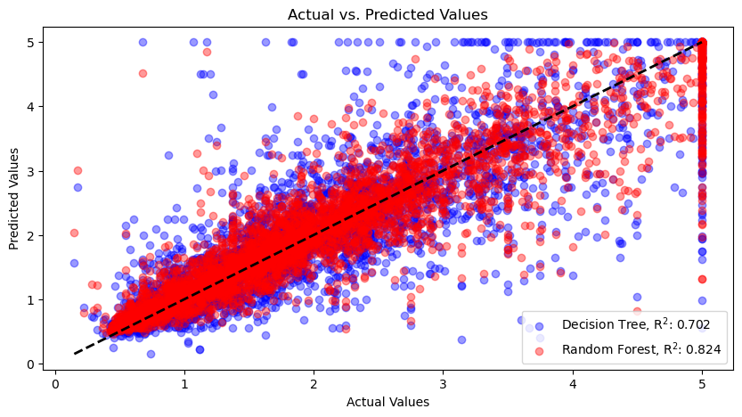 Actual values vs. predicted values for the decision tree (blue dots) and random forest (red dots) regressors. The dashed line represents the ideal scenario where the predicted values perfectly match the actual values. Points lying close to this line indicate accurate predictions, while points deviating from the line indicate discrepancies between the predicted and actual values. The random forest regressor performs better than the decision tree regressor, as indicated by the higher R-squared value.
The resulting plot shows the following:
- Actual Values (x-axis): Represents the actual target values from the test set. These are the true values of the target variable that we want to predict.
- Predicted Values (y-axis): Represents the predicted target values generated by the models. These are the values estimated by the decision tree and random forest models based on the input features.
- Scatter Plots: Points represent the relationship between the actual values and the predicted values. Each point corresponds to an instance in the test set. The blue points represent the predictions made by the decision tree model, and the red points represent the predictions made by the random forest model.
- Diagonal Black Dashed Line: Represents the ideal scenario where the predicted values perfectly match the actual values. Points lying close to this line indicate accurate predictions, while points deviating from the line indicate discrepancies between the predicted and actual values.
By examining the plot, you can visually assess how well the models are predicting the target variable. Ideally, the scatter plot points should cluster closely around the diagonal line. If the points deviate substantially from the line, it indicates that the model’s predictions are less accurate.
Additionally, the R-squared values annotated in the plot provide a quantitative measure of the model’s performance. The R-squared metric represents the proportion of the variance in the target variable that can be explained by the input features. A higher R-squared value (closer to 1) indicates a better fit between the predicted and actual values. As you can see, the random forest model performs better than the decision tree model, as indicated by the higher R-squared value.
Conclusion
In summary, decision trees and random forests are powerful machine learning algorithms used for classification and regression tasks. Decision trees provide interpretability but are prone to overfitting, while random forests mitigate this issue by aggregating multiple trees. Random forests offer better robustness to noisy data and outliers, but they are more complex and less interpretable than decision trees. In practice, random forests are often the preferred choice for classification and regression tasks due to their superior performance. However, decision trees are still useful in situations where interpretability is a priority.
The code for this post can be found in this GitHub repositoryꜛ
If you have any questions or suggestions, feel free to leave a comment below or reach out to me on Mastodonꜛ.

comments