Image denoising techniques: A comparison of PCA, kernel PCA, autoencoder, and CNN

In my previous posts, I discussed the application of PCA, factor analysis, and autoencoder for dimensionality reduction of high-dimensional datasets. However, such methods can also be utilized for other purposes such as image denoising. In this post, we will explore the potential of PCA, denoising autoencoders and Convolutional Neural Networks (CNN) for restoring noisy images using Python. We will examine their performance, advantages, and disadvantages to determine the most effective method for image denoising.

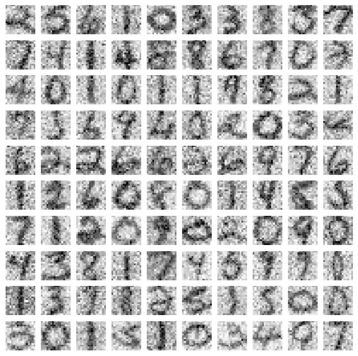
What is image denoising?

Image denoising refers to the process of reducing or removing unwanted noise from digital images. Noise in images can arise from various sources, such as sensor limitations, transmission interference, or environmental factors. The presence of noise can degrade image quality, blur details, and impact the accuracy of subsequent image analysis tasks. Image denoising techniques aim to restore the original content of the image by suppressing or eliminating the noise while preserving important image features and details. In this post, we will take a look at four different methods for image denoising, that I briefly introduce in the following.

Principal Component Analysis (PCA)

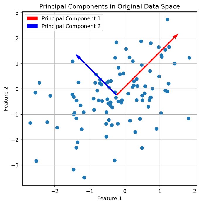Principle of PCA. Code to generate this figure can be found here.

PCA is a technique for dimensionality reduction that can also be applied to image denoising. By identifying the principal components of a dataset, PCA aims to capture the most significant information while discarding noise. Given a dataset $\mathbf{X}$ with $n$ samples and $d$ features, PCA seeks to find a lower-dimensional representation by projecting the data onto a new set of orthogonal axes, known as the principal components. This can be achieved by performing eigendecomposition on the covariance matrix of $\mathbf{X}$, \(\mathbf{C} = \frac{1}{n} \sum_{i=1}^{n} (\mathbf{x}_i - \boldsymbol{\mu})(\mathbf{x}_i - \boldsymbol{\mu})^T\), where $\mathbf{x}_i$ represents the $i$-th sample, and $\boldsymbol{\mu}$ is the mean vector of $\mathbf{X}$. The principal components are the eigenvectors corresponding to the largest eigenvalues of $\mathbf{C}$. In my previous post on PCA you can find some further details on how to calculate the principal components.

In the context of image denoising, PCA can effectively reduce noise by reconstructing images based on the retained principal components. By projecting the noisy image $\mathbf{Y}$ onto the principal components, the denoised image $\hat{\mathbf{X}}$ can be obtained as:

\[\hat{\mathbf{X}} = \mathbf{Y} \mathbf{V}_k \mathbf{V}_k^T\]

where $\mathbf{V}_k$ represents the matrix of the first $k$ principal components.

One advantage of PCA is its simplicity and interpretability, as the principal components can reveal the dominant patterns in the data. However, it may struggle to handle nonlinear relationships in the image data, which can limit its denoising performance in certain scenarios.

Kernel Principal Component Analysis (Kernel PCA)

Kernel PCA extends the capabilities of PCA by incorporating nonlinear mappings through kernel functions. Given a dataset $\mathbf{X}$ with $n$ samples and $d$ features, kernel PCA seeks to find a nonlinear transformation $\phi(\mathbf{x})$ that maps the data into a higher-dimensional feature space:

\[\phi: \mathbb{R}^d \rightarrow \mathcal{H}\]

where $\mathcal{H}$ represents the higher-dimensional feature space. The transformed data can then be linearly analyzed using PCA. Instead of computing the covariance matrix in the original feature space, the so-called kernel trickꜛ is applied, which involves calculating the inner products between the transformed samples,

\[\mathbf{K} = \begin{bmatrix} \langle \phi(\mathbf{x}_1), \phi(\mathbf{x}_1) \rangle & \langle \phi(\mathbf{x}_1), \phi(\mathbf{x}_2) \rangle & \cdots & \langle \phi(\mathbf{x}_1), \phi(\mathbf{x}_n) \rangle \\ \langle \phi(\mathbf{x}_2), \phi(\mathbf{x}_1) \rangle & \langle \phi(\mathbf{x}_2), \phi(\mathbf{x}_2) \rangle & \cdots & \langle \phi(\mathbf{x}_2), \phi(\mathbf{x}_n) \rangle \\ \vdots & \vdots & \ddots & \vdots \\ \langle \phi(\mathbf{x}_n), \phi(\mathbf{x}_1) \rangle & \langle \phi(\mathbf{x}_n), \phi(\mathbf{x}_2) \rangle & \cdots & \langle \phi(\mathbf{x}_n), \phi(\mathbf{x}_n) \rangle \\ \end{bmatrix}\]

where $\langle \cdot, \cdot \rangle$ denotes the inner product in the higher-dimensional feature space.

Kernel PCA can effectively remove noise from images by projecting them into this higher-dimensional feature space and applying PCA to the resulting kernel matrix $\mathbf{K}$. However, choosing an appropriate kernel function, such as the radial basis function (RBF) kernel, and tuning the hyperparameters can be challenging. Additionally, kernel PCA may also be computationally expensive, particularly for large image datasets due to the increased dimensionality of the feature space.

Autoencoder

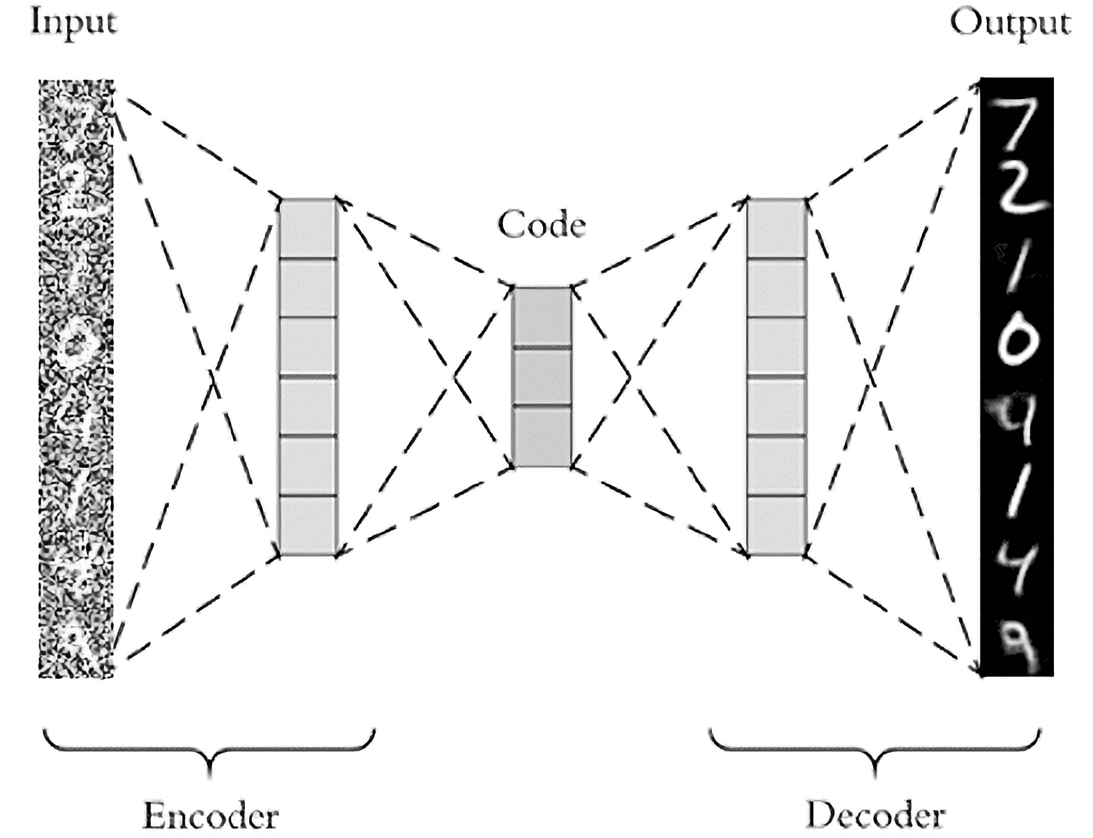
Architecture of an Autoencoder. Source: pyimagesearch.comꜛ

Autoencoders are neural networks designed to encode and decode data, making them suitable for image denoising tasks. Mathematically, an autoencoder consists of an encoder function $f_{\text{enc}}(\mathbf{X})$ that maps the input image $\mathbf{X}$ to a lower-dimensional latent space representation $\mathbf{h}$, and a decoder function $f_{\text{dec}}(\mathbf{h})$ that reconstructs the image from the latent representation. The encoder and decoder can be represented as:

\[\mathbf{h} = f_{\text{enc}}(\mathbf{X}) = \sigma(\mathbf{W}_{\text{enc}}\mathbf{x} + \mathbf{b}_{\text{enc}})\] \[\hat{\mathbf{X}} = f_{\text{dec}}(\mathbf{h}) = \sigma(\mathbf{W}_{\text{dec}}\mathbf{h} + \mathbf{b}_{\text{dec}})\]

where \(\mathbf{W}_\text{enc}\) and \(\mathbf{b}_\text{enc}\) represent the weights and biases of the encoder, \(\mathbf{W}_\text{dec}\) and \(\mathbf{b}_\text{dec}\) represent the weights and biases of the decoder, and \(\sigma(\cdot)\) denotes an activation function.

By training an autoencoder on noisy images $\hat{\mathbf{X}}$, the network learns to reconstruct the original, noise-free image $\mathbf{X}$, thus achieving the denoising effect. The autoencoder aims to learn a mapping that suppresses the noise while preserving essential image details.

Autoencoders excel at capturing intricate image features and can handle complex noise patterns. However, training an autoencoder requires a significant amount of computational resources, and obtaining optimal results may depend on choosing an appropriate architecture, such as the number of layers and hidden units, as well as tuning hyperparameters.

Convolutional Neural Network (CNN)

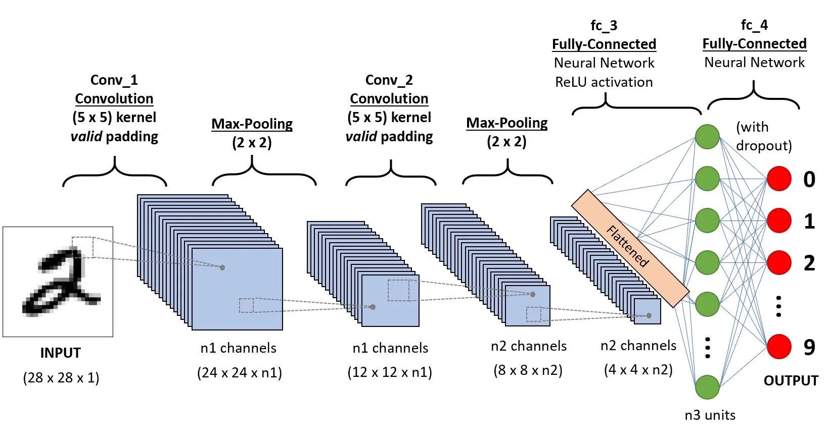Convolutional Neural Network (CNN) architecture. Sourceꜛ

Convolutional Neural Networks (CNNs) are widely used in image processing tasks, including image denoising. A CNN consists of multiple layers, including convolutional layers, pooling layers, and fully connected layers. The convolutional layers perform convolutions on the input image $\mathbf{X}$ using learnable filters (kernels) to extract local spatial features,

\[\mathbf{H} = \sigma(\mathbf{W} \ast \mathbf{X} + \mathbf{b})\]

where $\mathbf{H}$ is the feature map, $\sigma(\cdot)$ denotes an activation function, $\mathbf{W}$ represents the convolutional filters, and $\mathbf{b}$ is the bias term. The pooling layers then downsample the feature maps to capture the most salient information, which can be expressed as:

\[\mathbf{P} = \text{pooling}(\mathbf{H})\]

where $\mathbf{P}$ denotes the pooled feature map.

By leveraging their ability to capture spatial information through convolutions and pooling operations, CNNs can effectively restore noisy images. The hierarchical representations learned by CNNs allow them to discern noise from essential features, enabling robust denoising. CNNs are particularly adept at handling images with complex noise patterns due to their ability to capture and exploit local dependencies.

However, training CNNs for image denoising may require a large amount of annotated data, as they rely on supervised learning. Annotated data, consisting of pairs of noisy and clean images, is necessary for training the network to learn the denoising process effectively. Additionally, training CNNs for image denoising may involve longer training times due to the complexity of the network architecture and the size of the dataset. Despite these considerations, CNNs have demonstrated remarkable denoising capabilities and are widely employed in image denoising tasks.

Applying image denoising in Python

I will use the code from this sklearn tutorialꜛ as a starting point. This tutorial already included the application of PCA and kernel PCA, I will just add the application of the autoencoder and CNN. The tutorial is applied to the “Optical Recognition of Handwritten Digits” dataset, also known as the “United States Postal Service (USPS)” dataset, and consists of 9,298 16$\times$16 grayscale images of handwritten digits (Bakır et al. (2004)ꜛ). The dataset is provided by the sklearn OpenML libraryꜛ (here we use data id 41082). We split data into a training set and test set and add some Gaussian noise to both of them. To compare the performance of the different methods, we use the mean squared error (MSE, the lower the better) and the Peak-Signal-to-Noise Ratio (PSNR, the higher the better) as a metric:

import numpy as np
import matplotlib.pyplot as plt
from sklearn.decomposition import PCA
from tensorflow import keras
import tensorflow as tf
import random
from sklearn.datasets import fetch_openml
from sklearn.preprocessing import MinMaxScaler
from sklearn.model_selection import train_test_split
from sklearn.decomposition import PCA, KernelPCA

# for reproducibility:
random.seed(0)        # Python
np.random.seed(0)     # NumPy (which Keras uses)
tf.random.set_seed(0) # TensorFlow

# load sample data from OpenML and normalize it:
X, y = fetch_openml(data_id=41082, as_frame=False, return_X_y=True, parser="pandas")
X = MinMaxScaler().fit_transform(X)

# split the data into training and test sets:
X_train, X_test, y_train, y_test = train_test_split(
    X, y, stratify=y, random_state=0, train_size=1_000, test_size=100)

# add some noise to the data:
rng = np.random.RandomState(0)
noise_scale = 0.25
noise = rng.normal(scale=noise_scale, size=X_test.shape)
X_test_noisy = X_test + noise
noise = rng.normal(scale=noise_scale, size=X_train.shape)
X_train_noisy = X_train + noise

# calculate the MSE and PSNR for the noisy test image set:
max_I = X_test.max()
mse_noisy_image  = np.mean((X_test - X_test_noisy) ** 2)
psnr_noisy_image = 10 * np.log10(max_I / mse_noisy_image)

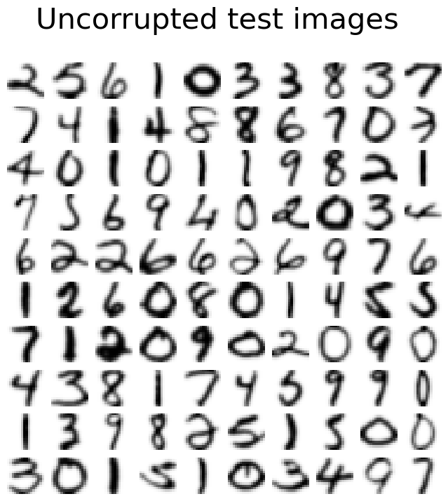
Let’s visualize the first 10 images of the test set:

def plot_digits(X, title):
    """helper function to plot 100 digits."""
    fig, axs = plt.subplots(nrows=10, ncols=10, figsize=(8, 8))
    for img, ax in zip(X, axs.ravel()):
        ax.imshow(img.reshape((16, 16)), cmap="Greys")
        ax.axis("off")
    fig.suptitle(title, fontsize=12)

plot_digits(X_test, "Uncorrupted test images")
plot_digits(X_test_noisy, f"Noisy test images\nMSE: {mse_noisy_image.round(2)}, PSNR: {psnr_noisy_image.round(2)} dB")

Uncorrupted test images.

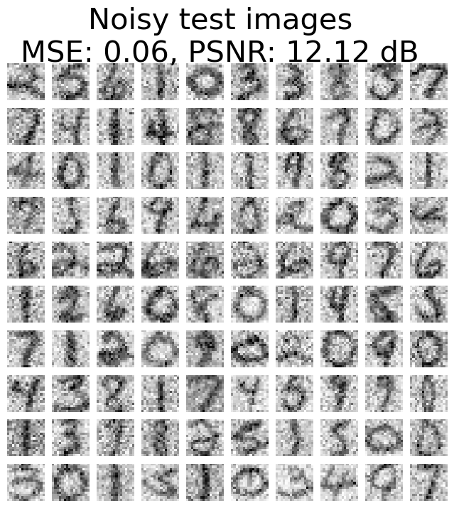Noisy test images. The MSE and PSNR of the noisy images are 0.06 and 12.2 dB, respectively.

Now we apply each of the methods to the noisy test images and compare the results.

PCA:

# PCA:
pca = PCA(n_components=32)
pca.fit(X_train_noisy)
X_reconstructed_pca = pca.inverse_transform(pca.transform(X_test_noisy))

# calculate the MSE and PSNR and plot:
mse_pca  = np.mean((X_test - X_reconstructed_pca) ** 2)
psnr_pca = 10 * np.log10(max_I / mse_pca)
plot_digits(X_reconstructed_pca,
            f"PCA reconstruction\nMSE: {mse_pca.round(2)}, PSNR: {psnr_pca.round(2)} dB")

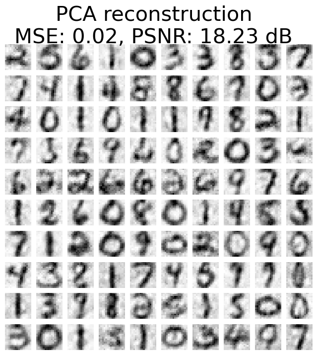PCA image reconstruction. The MSE and PSNR of the noisy images are 0.02 and 18.23 dB, respectively.

Kernel PCA:

# Kernel PCA:
kernel_pca = KernelPCA(n_components=400, kernel="rbf", gamma=1e-3, 
                       fit_inverse_transform=True, alpha=5e-3 )
_ = kernel_pca.fit(X_train_noisy)
X_reconstructed_kernel_pca = kernel_pca.inverse_transform(kernel_pca.transform(X_test_noisy))

# calculate the MSE and PSNR and plot:
mse_kernel_pca  = np.mean((X_test - X_reconstructed_kernel_pca) ** 2)
psnr_kernel_pca = 10 * np.log10(max_I / mse_kernel_pca)
plot_digits(X_reconstructed_kernel_pca,
            f"Kernel PCA reconstruction\n MSE: {mse_kernel_pca.round(2)}, PSNR: {psnr_kernel_pca.round(2)} dB")

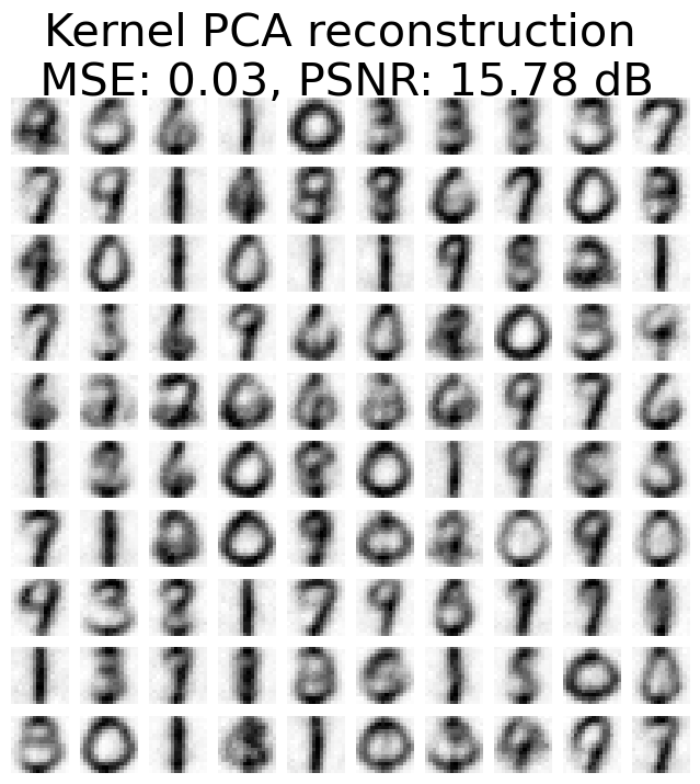Kernel PCA image reconstruction. The MSE and PSNR of the noisy images are 0.03 and 15.78 dB, respectively.

Autoencoder:

# define the Autoencoder model architecture
autoencoder = keras.models.Sequential([
    keras.layers.Dense(256, activation='relu', input_shape=(X_train.shape[1],)),
    keras.layers.Dense(128, activation='relu'),
    keras.layers.Dense(64, activation='relu'),
    keras.layers.Dense(128, activation='relu'),
    keras.layers.Dense(256, activation='relu'),
    keras.layers.Dense(X_train.shape[1])])

# compile and train the Autoencoder
autoencoder.compile(optimizer='adam', loss='mse')
autoencoder.fit(X_train_noisy, X_train, epochs=10, batch_size=32)

# apply denoising using Autoencoder:
X_reconstructed_autoencoder = autoencoder.predict(X_test_noisy)

# calculate the MSE and PSNR and plot:
mse_ae  = np.mean((X_test - X_reconstructed_autoencoder) ** 2)
psnr_ae = 10 * np.log10(max_I / mse_ae)
plot_digits(X_reconstructed_autoencoder,
            f"Autoencoder reconstruction\nMSE: {mse_ae.round(2)}, PSNR: {psnr_ae.round(2)} dB")

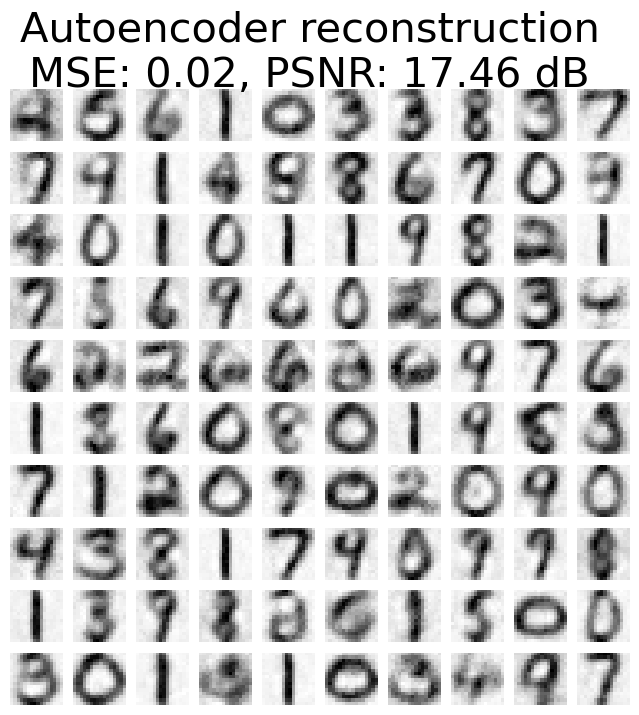Autoencoder image reconstruction. The MSE and PSNR of the noisy images are 0.02 and 17.46 dB, respectively.

CNN:

# define the CNN model architecture:
cnn = keras.models.Sequential([
    keras.layers.Reshape((16, 16, 1), input_shape=(256,)),
    keras.layers.Conv2D(32, (3, 3), activation='relu', padding='same'),
    keras.layers.Conv2D(64, (3, 3), activation='relu', padding='same'),
    keras.layers.Conv2D(1, (3, 3), activation='sigmoid', padding='same'),
    keras.layers.Reshape((256,))])

# compile and train the CNN:
cnn.compile(optimizer='adam', loss='mse')
cnn.fit(np.expand_dims(X_train_noisy, axis=-1), X_train, epochs=10, batch_size=32)

# apply denoising using CNN:
X_reconstructed_cnn = cnn.predict(np.expand_dims(X_test_noisy, axis=-1))

# calculate the MSE and PSNR and plot:
mse_cnn  = np.mean((X_test - X_reconstructed_cnn) ** 2)
psnr_cnn = 10 * np.log10(max_I / mse_cnn)
plot_digits(X_reconstructed_cnn,
            f"CNN reconstruction\nMSE: {mse_cnn.round(2)}, PSNR: {psnr_cnn.round(2)} dB")

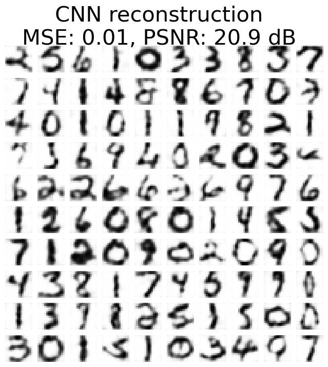CNN image reconstruction. The MSE and PSNR of the noisy images are 0.01 and 20.9 dB, respectively.

So, which method performs better for the given set of noisy images? The direct comparison of PCA and Kernel PCA shows, that PCA has a lower mean squared error (MSE) and higher peak signal-to-noise ratio (PSNR), indicating better reconstruction performance. However, the visual inspection of the reconstructed images shows, that Kernel PCA may preserve image features better.

The same comparison can be made between the autoencoder and PCA. It is important to note that the autoencoder and PCA have the same MSE, which would indicate equally good performance for both methods. However, the autoencoder has a lower PSNR, suggesting lower performance compared to PCA.

The best performance is achieved with the Convolutional Neural Network (CNN). The reconstructed images from the CNN are qualitatively very close to the uncorrupted images and have the lowest MSE and highest PSNR among all the methods. As mentioned above, CNNs are known to be very effective in capturing spatial information, which is crucial for image denoising. But this comes at a cost: CNNs are computationally expensive and require in general a larger amount of training data.

Conclusion

In conclusion, CNNs are the most effective method for image denoising, but they come with computational and data requirements. PCA and Kernel PCA provide simple yet effective denoising capabilities, while denoising autoencoders leverage neural networks to capture complex image features. Choosing the most suitable method for image denoising depends on factors such as the nature of noise, available computational resources, available amount of training data, and the desired level of denoising performance. By understanding the strengths and limitations of each technique, we can make better decisions when applying these methods to enhance the quality of images.

Please let me know, which experience you have made with image denoising and which methods you would recommend. Feel free to leave a comment below or reach out to me on Mastodonꜛ.

Here are some further reading recommendations on the methods applied in this post:

• Paper by Bakır et al. (2004)ꜛ on Kernel PCA and the USPS dataset
• Wikipedia article on Kernel PCAꜛ
• Wikipedia article on autoencoders and denoising autoencodersꜛ
• pyimagesearch.com on denoising autoencodersꜛ
• analyticsvidhya.com on denoising autoencodersꜛ
• CNN on towardsdatascience.comꜛ

The entire code used in this post is also available in this GitHub repositoryꜛ.