Using Autoencoders to reveal hidden structures in high-dimensional data

Autoencoders are a type of artificial neural network used for learning efficient representations of data, typically for the purpose of dimensionality reduction. They work by encoding the data, compressing it into a so-called latent or encoded space representation, and then reconstructing the data back from this compressed representation. In this Python tutorial, we discuss the use of Autoencoders in dimensionality reduction and how this can help us uncover hidden patterns in our data.

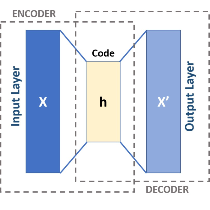
Schematic of a three-layered Autoencoder. CC BY-SA 4.0 (wikimedia.orgꜛ)

The concept of a Autoencoders

An autoencoder is a neural network that is trained unsupervised (i.e., no annotated data is required in advance) to learn an efficient and compressed representation of the input data. Mathematically, an autoencoder can be represented as a function $f$ that maps an input $x$ to a reconstruction $\hat{x}$:

\[h = f(x)\] \[\hat{x} = g(h)\]

Here $f$ is the encoder and $g$ is the decoder. The encoder compresses the input data into a low-dimensional representation $h$, and the decoder reconstructs the data from this representation. The goal of the autoencoder is to make the reconstruction $\hat{x}$ as close as possible to the original input $x$ such that the reconstruction error $||x-\hat{x}||$ is minimized. Autoencoders are trained by minimizing a loss function (e.g., mean squared error) between the input and the output of the network.

The encoder $f$ and the decoder $g$ consist of several layers of neurons interconnected using linear transformations and nonlinear activation functions. In the simplest case, an autoencoder consists of three layers as depicted in the header image of this post. These layers are:

1. Input layer: This is the first layer of the autoencoder and is defined by an encoding function. The shape of the input layer is determined by the number of features (to be specified).
2. Hidden layer (encoding layer or encoded space): This layer is defined by $N_\text{dim}$ neurons and an activation function, e.g., the ReLU (Rectified Linear Unit) function. $N_\text{dim}$ is the number of encoding dimensions (to be specified) in the encoded space, which thus corresponds to the number on the dimensions to be reduced. In this layer, the input data are encoded and reduced to a few “factors” or neurons.
3. Output layer: This layer is defined by $N_\text{feat-dim}$ neurons and an activation function, e.g., the sigmoid function. $N_\text{feat-dim}$ also corresponds to the number of features. The output layer reconstructs the data by trying to generate an approximation of the input.

You may now ask, why do we need the output layer if we are only interested in the encoded space? The answer is that the output layer is needed to train the autoencoder. As mentioned above, the autoencoder is trained by minimizing the reconstruction error between the input and the output of the network. The output layer is thus needed to reconstruct the input data from the encoded space. When the autoencoder model is well trained, the output layer can be discarded.

Autoencoder in Python: Wine dataset example

As for the PCA and Factor Analysis example , we will use the high-dimensional “Wine” datasetꜛ from the sklearn-datasets library. Please refer to these posts for basic details about the dataset, I will skip the introduction here.

Again, let’s import the relevant packages and load and normalize the dataset first:

import numpy as np
import pandas as pd
import matplotlib.pyplot as plt
import seaborn as sns
from sklearn.datasets import load_wine
from sklearn.preprocessing import StandardScaler
from tensorflow.keras.models import Model
from tensorflow.keras.layers import Input, Dense
from sklearn.model_selection import train_test_split
import tensorflow as tf
from keras import regularizers
from tensorflow.keras.optimizers import Adam
import random
from sklearn.cluster import DBSCAN, KMeans

# load the toy data: 
input_data = load_wine()
X = input_data.data

# normalize the data: 
X_Factor = StandardScaler().fit_transform(X)
df = pd.DataFrame(data=X_Factor, columns=input_data.feature_names)

df_full = df.copy()
df_full['Target'] = input_data.target
target_names = input_data.target_names

Next, we will create the autoencoder model. We will use the Dense() function from the keras package to create the input, encoding, and decoding layers. The Dense() function creates a fully-connected layer with the specified number of neurons and activation function. As mentioned above, the number of neurons in the input layer (num_features) is determined by the number of features in the dataset. The number of neurons in the encoding layer (encoding_dim) is determined by the number of dimensions of the latent space to encode. The number of neurons in the decoding layer is then again determined by the number of features in the dataset. The activation function of the encoding layer is typically the ReLU activation function ('relu'), and the activation function of the decoding layer is typically the sigmoid activation function (sigmoid). The autoencoder model (autoencoder) is created using the Model() function, also again from the keras package. The Model() function takes the input layer and the output layer as arguments:

# for reproducibility:
random.seed(0)        # Python
np.random.seed(0)     # NumPy (which Keras uses)
tf.random.set_seed(0) # TensorFlow

# determine the number of features:
num_features = X_Factor.shape[1]

# define the number of dimensions of the (latent) space to encode:
encoding_dim = 3

# create the input layer:
input_layer = input(shape=(num_features,))

# create the encoding layer:
encoded = Dense(encoding_dim, activation='relu')(input_layer)

# create the decoding layer:
decoded = Dense(num_features, activation='sigmoid')(encoded)

# create the autoencoder model:
autoencoder = Model(inputs=input_layer, outputs=decoded)

Info
Neural networks, including autoencoders, involve a significant amount of randomness. This comes from two primary sources:

1. Weight Initialization: The initial values for the weights and biases in the network are typically set randomly. This means that each time you create a new model, it starts from a different place.
2. Mini-Batch Gradient Descent: During training, the data is usually divided into mini-batches, and the order of the batches affects the learning process. This order is typically randomized each epoch.

To get consistent results from run to run, we can set a seed for the random number generator that controls these processes. This is the reason for the random.seed(0), np.random.seed(0), and tf.random.set_seed(0) commands in the code above. Note that this does not guarantee identical results from run to run, but it does make the results more consistent and repeatable.

We then compile the autoencoder model using the compile() function from the keras package. The compile() function takes the optimizer and the loss function as arguments. The autoencoder model is then trained using the fit() function, which takes the input data, the output data, the number of epochs, the batch size, and the shuffle argument as arguments:

# compile and train the model:
autoencoder.compile(optimizer='adam', loss='mse')
autoencoder.fit(X_Factor, X_Factor, epochs=100, batch_size=16, 
                shuffle=True)

Next, we can use the trained autoencoder model to encode the input data. We can do this by creating an encoder model (encoder) that takes the input data and returns the encoded data (encoded_data). The encoder model is created again using the Model() function, this time taking the input layer and the encoding layer as arguments. The encoder model is then applied to the input data (X_Factor) using the predict() function, which returns the encoded data:

# create an encoder model:
encoder = Model(inputs=input_layer, outputs=encoded)

# apply the encoder to the input data:
encoded_data = encoder.predict(X_Factor)

For convenience, we create a DataFrame for the encoded data and add the target values (wine classes) to it:

# create a DataFrame for the encoded data:
df_encoded = pd.DataFrame(data=encoded_data, 
              columns=['Feature 1', 'Feature 2', 'Feature 3'])
df_encoded['Target'] = input_data.target

That’s it! The encoded data is our reduced dataset and can now be used for further analysis. Let’s plot the encoded data:

# visualization of coded data (i.e. latent variables, here called "Features"):
colors = ['r', 'g', 'b']
fig = plt.figure()
ax = fig.add_subplot(111, projection='3d')
for target, color in zip(target_names, colors):
    indices = df_encoded['Target'] == input_data.target_names.tolist().index(target)
    ax.scatter(df_encoded.loc[indices, 'Feature 1'], 
               df_encoded.loc[indices, 'Feature 2'],
               df_encoded.loc[indices, 'Feature 3'], c=color, label=target)
ax.view_init(elev=35, azim=45)
ax.set_xlabel('Feature 1')
ax.set_ylabel('Feature 2')
ax.set_zlabel('Feature 3', rotation=90)
ax.zaxis.labelpad=-4.9
ax.set_title('Autoencoder Encoding of Wine Dataset')
ax.legend()
plt.show()

fig, axs = plt.subplots(1, 3, figsize=(12, 4))  # Adjust the figure size as needed
# XY projection: 
for target, color in zip(target_names, colors):
    indices = df_encoded['Target'] == input_data.target_names.tolist().index(target)
    axs[0].scatter(df_encoded.loc[indices, 'Feature 1'], df_encoded.loc[indices, 'Feature 2'], c=color, label=target)
axs[0].set_xlabel('Feature 1')
axs[0].set_ylabel('Feature 2')
axs[0].set_title('XY Projection')

# XZ projection:
for target, color in zip(target_names, colors):
    indices = df_encoded['Target'] == input_data.target_names.tolist().index(target)
    axs[1].scatter(df_encoded.loc[indices, 'Feature 1'], df_encoded.loc[indices, 'Feature 3'], c=color, label=target)
axs[1].set_xlabel('Feature 1')
axs[1].set_ylabel('Feature 3')
axs[1].set_title('XZ Projection')

# YZ projection:
for target, color in zip(target_names, colors):
    indices = df_encoded['Target'] == input_data.target_names.tolist().index(target)
    axs[2].scatter(df_encoded.loc[indices, 'Feature 2'], df_encoded.loc[indices, 'Feature 3'], c=color, label=target)
axs[2].set_xlabel('Feature 2')
axs[2].set_ylabel('Feature 3')
axs[2].set_title('YZ Projection')
plt.show()

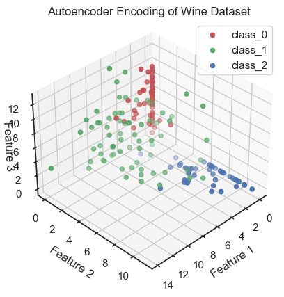
Autoencoder (3D view): Coding data and reduction to three latent variables (here called “features”). The three latent variable span the so-called latent space, also called the “code space” or “feature space”.

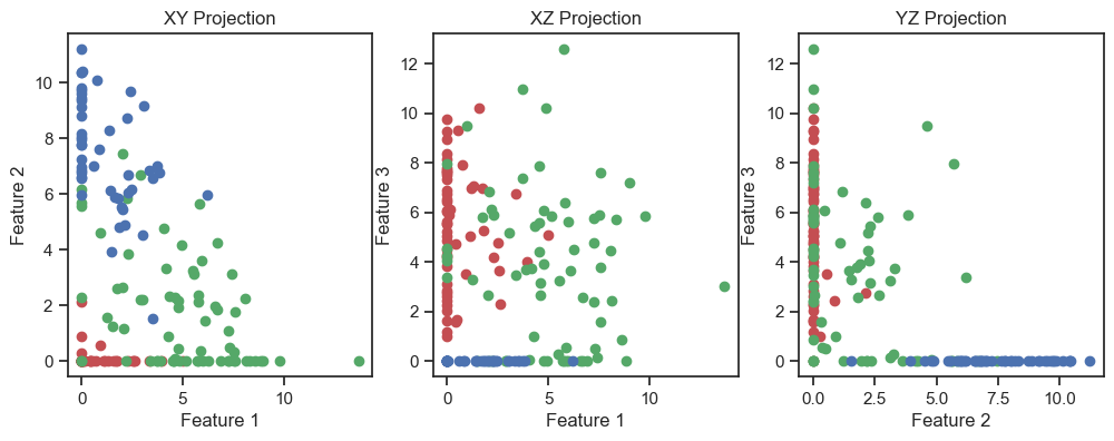Autoencoder (2D projections), similar to the image above.

Interpretation of the latent variables

To make a (vague) interpretation of the latent variables, we can look at the weights between the neurons from the input layer and those from the hidden/encoded layer. The weights indicate how much each feature contributes to building the coded representation of the data:

hidden_layer_weights = autoencoder.layers[1].get_weights()[0]

# for convenience, we create a DataFrame for the weights:
df_weights = pd.DataFrame(data=hidden_layer_weights, 
                columns=['Factor 1', 'Factor 2', 'Factor 3'], 
                index=feature_names)

# visualize the weights:
fig, axs = plt.subplots(nrows=int(np.ceil(num_features/3)), ncols=3, figsize=(8, 11))
for i, feature in enumerate(feature_names):
    ax = axs[i//3, i%3]
    weights = df_weights.loc[feature].values
    factors = ['Factor 1', 'Factor 2', 'Factor 3']
    colors = ['grey' if w < 0 else 'blue' for w in weights]
    ax.bar(factors, weights, color=colors)
    ax.set_xlabel('Factor')
    ax.set_ylabel('Weight')
    ax.set_title(f'Autoencoder Weights for\n {feature}')
plt.tight_layout()
plt.show()

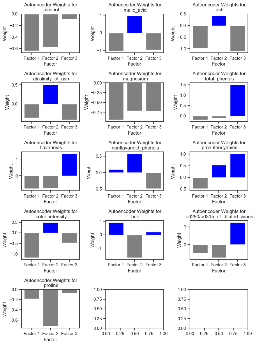
Autoencoder weights for each feature in the Wine dataset. The weights indicate how much each feature contributes to building the coded representation of the data in the dataset.

Additionally and for convenience, we filter the features with positive weights for each factor:

# filter the features with positive weights for each factor
positive_features = {}
for factor in df_weights.columns:
    positive_features[factor] = df_weights.index[df_weights[factor] > 0].tolist()

# output of the features with positive weights for each factor:
for factor, features in positive_features.items():
    print(f"Features with positive weights for {factor}:")
    print(features)
    print()

Features with positive weights for Factor 1:
['nonflavanoid_phenols', 'hue']

Features with positive weights for Factor 2:
['malic_acid', 'ash', 'alcalinity_of_ash', 'nonflavanoid_phenols', 'proanthocyanins', 'color_intensity']

Features with positive weights for Factor 3:
['total_phenols', 'flavanoids', 'proanthocyanins', 'hue', 'od280/od315_of_diluted_wines']

As we can see, the latent variables are not directly related to the original features. Instead, they are a combination of the original features:

• the first latent variable is a combination of the nonflavanoid_phenols and hue features.
• the second latent variable is a combination of the malic_acid, ash, alcalinity_of_ash, nonflavanoid_phenols, proanthocyanins, and color_intensity features, while
• the third latent variable is a combination of the total_phenols, flavanoids, proanthocyanins, hue, and od280/od315_of_diluted_wines.

The features ‘alcohol’, ‘proline’ and ‘magnesium’ had no positive weights for any of the latent variables, i.e., they were not important for the autoencoder to reconstruct the data.

This is just a very rough interpretation of the latent variables. In general, it is not always possible to interpret the latent variables in a meaningful way. However, we can use the latent variables, e.g., for further classification of the data, as we will see in the next section.

Verification of the correspondence of the factors with the real classes

As we have done for the PCA and Factor Analysis example, we can check whether the latent variables are related to the real classes in the dataset. To do so, we try to re-identify the three wine classes within the latent space by clustering the latent variables once with DBSCAN and once with Kmeans:

""" Verify reproducibility by "blindly" (unsupervised) 
identifying clusters from the latent variables (i.e., do the 
clusters match with the actual classes?): """
dbscan = DBSCAN(eps=1.80, min_samples=5)
dbscan_labels = dbscan.fit_predict(np.array(encoded_data))
dbscan_labels_unique = set(dbscan_labels)

fig = plt.figure()
ax = fig.add_subplot(111, projection='3d')
for label in dbscan_labels_unique:
    if label ==-1:
        cluster_points = np.array(encoded_data)[dbscan_labels==label]
        ax.scatter(cluster_points[:,0], cluster_points[:,1], cluster_points[:,2], marker="x", 
                   label="Noise", color="grey")
    else:
        cluster_points = np.array(encoded_data)[dbscan_labels==label]
        ax.scatter(cluster_points[:,0], cluster_points[:,1], cluster_points[:,2], 
                   label=f"Cluster {label+1}")
ax.view_init(elev=35, azim=45)
ax.set_xlabel('Factor 1')
ax.set_ylabel('Factor 2')
ax.set_zlabel('Factor 3')
ax.set_title('DBSCAN Clustering of the latent variables')
ax.zaxis.labelpad=-3.9
ax.legend()
plt.show()
        
fig, axs = plt.subplots(1, 3, figsize=(12, 4))  # Adjust the figure size as needed
# XY projection:
for label in dbscan_labels_unique:
    if label ==-1:
        cluster_points = np.array(encoded_data)[dbscan_labels==label]
        axs[0].scatter(cluster_points[:,0], cluster_points[:,1], marker="x", 
                   label="Noise", color="grey")
    else:
        cluster_points = np.array(encoded_data)[dbscan_labels==label]
        axs[0].scatter(cluster_points[:,0], cluster_points[:,1], 
                   label=f"Cluster {label+1}")
axs[0].set_xlabel('Factor 1')
axs[0].set_ylabel('Factor 2')
axs[0].set_title('DBSCAN classes XY Projection')
# XZ projection:
for label in dbscan_labels_unique:
    if label ==-1:
        cluster_points = np.array(encoded_data)[dbscan_labels==label]
        axs[1].scatter(cluster_points[:,0], cluster_points[:,2], marker="x", 
                   label="Noise", color="grey")
    else:
        cluster_points = np.array(encoded_data)[dbscan_labels==label]
        axs[1].scatter(cluster_points[:,0], cluster_points[:,2], 
                   label=f"Cluster {label+1}")
axs[1].set_xlabel('Factor 1')
axs[1].set_ylabel('Factor 3')
axs[1].set_title('DBSCAN classes XZ Projection')
# YZ projection:
for label in dbscan_labels_unique:
    if label ==-1:
        cluster_points = np.array(encoded_data)[dbscan_labels==label]
        axs[2].scatter(cluster_points[:,1], cluster_points[:,2], marker="x", 
                   label="Noise", color="grey")
    else:
        cluster_points = np.array(encoded_data)[dbscan_labels==label]
        axs[2].scatter(cluster_points[:,1], cluster_points[:,2], 
                   label=f"Cluster {label+1}")
axs[2].set_xlabel('Factor 2')
axs[2].set_ylabel('Factor 3')
axs[2].set_title('DBSCAN classes YZ Projection')
plt.show()

and

kmeans = KMeans(n_clusters=3, random_state=0)
kmeans_labels = kmeans.fit_predict(np.array(encoded_data))
kmeans_labels_unique = set(kmeans_labels)

fig = plt.figure()
ax = fig.add_subplot(111, projection='3d')
for label in kmeans_labels_unique:
    cluster_points = encoded_data[kmeans_labels==label]
    ax.scatter(cluster_points[:,0], cluster_points[:,1], cluster_points[:,2], 
                   label=f"Cluster {label+1}")
ax.view_init(elev=35, azim=45)
ax.set_xlabel('Factor 1')
ax.set_ylabel('Factor 2')
ax.set_zlabel('Factor 3')
ax.set_title('KMEANS Clustering of the Factors')
ax.zaxis.labelpad=-3.9
ax.legend()
plt.show()
        
fig, axs = plt.subplots(1, 3, figsize=(12, 4))  # Adjust the figure size as needed
# XY projection:
for label in kmeans_labels_unique:
    cluster_points = encoded_data[kmeans_labels==label]
    axs[0].scatter(cluster_points[:,0], cluster_points[:,1], 
                   label=f"Cluster {label+1}")
axs[0].set_xlabel('Factor 1')
axs[0].set_ylabel('Factor 2')
axs[0].set_title('KMEANS classes XY Projection')
# XZ projection:
for label in kmeans_labels_unique:
    cluster_points = encoded_data[kmeans_labels==label]
    axs[1].scatter(cluster_points[:,0], cluster_points[:,2], 
                   label=f"Cluster {label+1}")
axs[1].set_xlabel('Factor 1')
axs[1].set_ylabel('Factor 13')
axs[1].set_title('KMEANS classes XZ Projection')
# YZ projection:
for label in kmeans_labels_unique:
    cluster_points = encoded_data[kmeans_labels==label]
    axs[2].scatter(cluster_points[:,1], cluster_points[:,2], 
                   label=f"Cluster {label+1}")
axs[2].set_xlabel('Factor 2')
axs[2].set_ylabel('Factor 3')
axs[2].set_title('KMEANS classes YZ Projection')
plt.show()

3D scatter plots: Top: Latent variables with color-assignments regarding the original classes. Bottom left: DBSCAN clustering of the latent variables. Bottom right: Kmeans clustering of the latent variables.

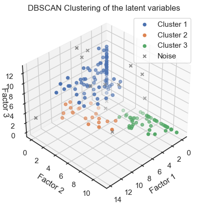
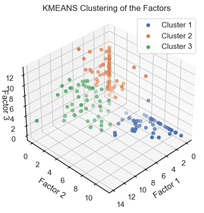
Latent variables with color-assignments regarding the original classes (2D projections).

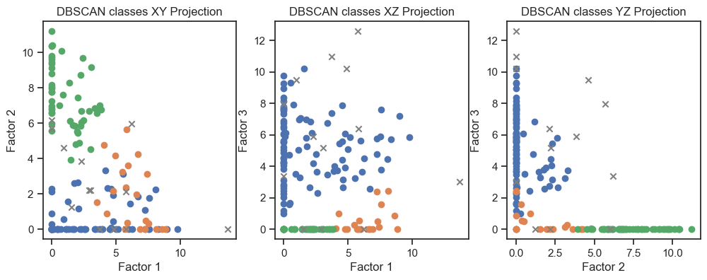DBSCAN clustering of the latent variables. (2D projections).

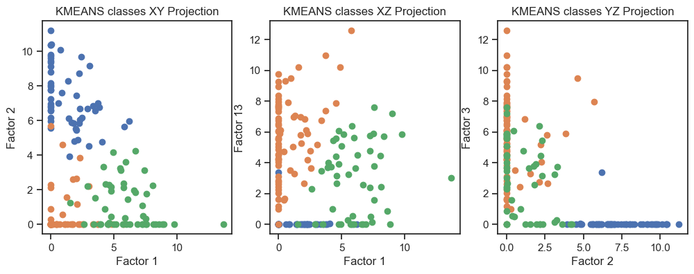Kmeans clustering of the latent variables. (2D projections).

We can see that the clustering of the latent variables is not that accurate in re-identifying the classes of the original data. This is expected since the latent variables are a compressed version of the original data. However, we can see that the clustering of the latent variables is not bad at all. The DBSCAN clustering is not as good as the Kmeans clustering. This is expected as DBSCAN is a density-based clustering algorithm and the latent variables are not as dense as the original data.

Validation of the Autoencoder model

When we trained the model, we actually skipped some crucial steps. First, we did not validate the model. Second, we trained the model on the whole dataset. However, we should always validate our model to make sure that it is not overfitting. To do so, we need some kind of metric to measure the performance of the model. Such metric is the loss function. The loss function is a measure of how well the model is able to reconstruct the original data. The fit() function in our example above also returns a so-called history object, that contains the loss values for each epoch. Let’s have a look at it:

Inspecting the loss curve

random.seed(0)        # Python
np.random.seed(0)     # NumPy (which Keras uses)
tf.random.set_seed(0) # TensorFlow

# plot the loss over epochs:
history = autoencoder.fit(X_Factor, X_Factor, 
            epochs=200, batch_size=16, shuffle=True, 
            verbose=0)
plt.figure(figsize=(6,4))
plt.plot(history.history['loss'])
plt.title('Model loss')
plt.ylabel('Loss')
plt.xlabel('Epoch')
plt.legend(['Train'], loc='upper right')
plt.show()

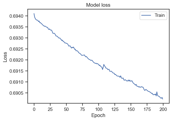Model loss for the entire dataset.

Please note, that I’ve increased the number of epochs to 200. We can see that the loss is decreasing over epochs, but doesn’t stabilize. To get a general idea, how to interpret a loss curve, there are some rules of thumb:

• Decreasing Loss: At the beginning of the training process, the model is not yet well adjusted to represent the data, so the loss will likely be high. As epochs pass and the model continues to learn from the data, the loss should decrease. This illustrates that the model is improving its ability to reconstruct the original data from the encoded form.
• Stabilization: After a certain number of epochs, the loss curve might start to flatten, indicating that the model isn’t improving significantly from additional training. This can mean that the model has essentially learned the underlying patterns in the data, and further training would not significantly reduce the loss.
• Overfitting: If training continues for too many epochs, the loss might start to increase. This is typically a sign of overfitting, where the model begins to “memorize” the training data and lose its ability to generalize to unseen data.

Our loss curve doesn’t stabilize. And at first glance, the curve seems to show a decreasing loss. However, taking a closer look at the scaling of the y-axis, we can see that this is only a minor decrease. In fact, our loss curve is very flat. Also, it is not clear if the loss would continue to “decrease” or if it would flatten out after some more epochs. To get a better idea, we can introduce a validation set. The validation set is a subset of the training data that is not used for training. Instead, it is used to evaluate the model’s performance on unseen data. To get such validation set, we need split our dataset:

Splitting the dataset into training and validation sets

For example, a common approach is to split the dataset into a 80-20 or 70-30 split for training and validation. In the following, we will use a 80-20 split:

# split the dataset into training and testing sets:
X_train, X_val = train_test_split(X_Factor, test_size=0.2,
                                  random_state=0)

Let’s repeat the training process, but this time we will use the validation set to evaluate the model’s performance:

random.seed(0)        # Python
np.random.seed(0)     # NumPy (which Keras uses)
tf.random.set_seed(0) # TensorFlow

autoencoder = Model(inputs=input_layer, outputs=decoded)
autoencoder.compile(optimizer='adam', loss='mse')
history = autoencoder.fit(X_train, X_train, 
                          validation_data=(X_val, X_val), 
                          epochs=200, batch_size=16)

# plot the updated loss curve:
plt.figure(figsize=(6,4))
plt.plot(history.history['loss'], label='Train Loss')
plt.plot(history.history['val_loss'], label='Validation Loss')
plt.title('Model loss')
plt.ylabel('Loss')
plt.xlabel('Epoch')
plt.legend(loc='upper right')
plt.show()

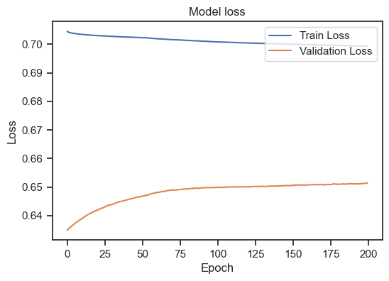Model loss for the training and validation set.

We can see, that the training loss is still (slightly) decreasing, but the validation loss is increasing. This is a clear sign of overfitting. To get a general idea, how to interpret the training loss together with the validation loss, there are again some rules of thumb:

• Overfitting: If the loss on the training data set continues to decrease, but the loss on the validation data set increases or stagnates, this may be a sign of overfitting. The model is memorizing the training data too well and may be interfering with generalization on new data.
• Underfitting: If the loss on both the training data set and the validation data set is high or stagnant, this indicates underfitting. The model may not have sufficient capacity to capture the structure of the data and may not generalize well to the training or validation data.
• Good model: A good model indicates a decrease in loss on both datasets, with the loss on the validation dataset similar to or slightly higher than the loss on the training dataset. This indicates that the model learns well on the training data while having the ability to generalize on the validation data.

So, in our case, the model is not able to generalize to unseen data. To improve our model, there are several options:

Improving the model

There are several measures, how we can improve a model:

• Model Complexity: The model might not be complex enough to capture the underlying patterns in the data. We could try increasing the complexity of the model, perhaps by adding more layers or nodes in the layers, or by trying different activation functions.
• Learning Rate: The learning rate might not be set appropriately. If it’s too high, the model might be overshooting the minimum; if it’s too low, the learning could be too slow or get stuck in a local minimum.
• Epochs: The number of epochs could be insufficient. It might be the case that the model simply needs more time to learn.
• Overfitting: Overfitting can occur if the model is too complex and begins to “memorize” the training data. If the training loss is much lower than the validation loss, this might be the case. Regularization techniques (like dropout, L1/L2 regularization) can help prevent this.
• Data Preprocessing: Our data might require additional preprocessing. Normalizing or standardizing the input data, if not already done, could improve the model’s performance.
• Outliers: Outliers in your data can significantly impact the performance of our model. Check for outliers and consider handling them, if they exist.
• Alternate Optimizer: We may also experiment with different optimizers. RMSProp, Adam, SGD with momentum are some commonly used ones.

In the following we will try some of the suggested measures:

Regularization

We regularize the model by adding a L1 regularization term to the encoding layer:

# the model is overfitting. Let's try to regularize it:
random.seed(0)        # Python
np.random.seed(0)     # NumPy (which Keras uses)
tf.random.set_seed(0) # TensorFlow

# create the encoding layer with L1 regularization
encoded = Dense(encoding_dim, activation='relu', 
                activity_regularizer=regularizers.l1(10e-5))(input_layer)
# create the decoding layer
decoded = Dense(num_features, activation='sigmoid')(encoded)

# create the autoencoder model
autoencoder = Model(inputs=input_layer, outputs=decoded)

# compile the model
autoencoder.compile(optimizer='adam', loss='mse')

# train the model:
history = autoencoder.fit(X_train, X_train, 
                          validation_data=(X_val, X_val), 
                          epochs=200, batch_size=16, shuffle=True)

# plot the updated loss curve:
plt.figure(figsize=(6,4))
plt.plot(history.history['loss'], label='Train Loss')
plt.plot(history.history['val_loss'], label='Validation Loss')
plt.title('Model loss')
plt.ylabel('Loss')
plt.xlabel('Epoch')
plt.legend(loc='upper right')
plt.show()

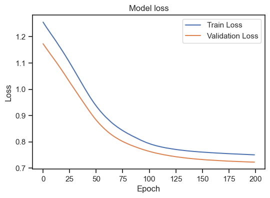Model loss for the training and validation set with L1 regularization.

As we can see, the regularization indeed improves the model as both curves are now decreasing. The model could be considered as “good model” by our above definition.

Changing the learning rate

Let’s see, how changing the learning rate affects the model:

# change the learning rate:
random.seed(0)        # Python
np.random.seed(0)     # NumPy (which Keras uses)
tf.random.set_seed(0) # TensorFlow

# specify the learning rate:
lr = 1 #0.001 default

# create an Adam optimizer with the given learning rate_
optimizer = Adam(lr=lr)

# compile and train the model:
autoencoder.compile(optimizer=optimizer, loss='mse')
history = autoencoder.fit(X_train, X_train, validation_data=(X_val, X_val), epochs=200, batch_size=16, shuffle=True)

# plot the updated loss curve:
plt.figure(figsize=(6,4))
plt.plot(history.history['loss'], label='Train Loss')
plt.plot(history.history['val_loss'], label='Validation Loss')
plt.title('Model loss')
plt.ylabel('Loss')
plt.xlabel('Epoch')
plt.legend(loc='upper right')
plt.show()

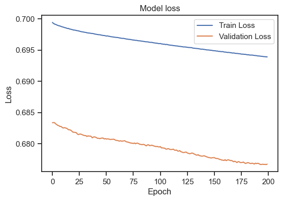Model loss for the training and validation set with a different learning rate.

With a learning rate of 1, we worsen our model. Training loss and validation loss diverge. I stop here, but you can play around with different learning rates. Selecting a good learning rate is highly dependent on the specific details of the underlying machine learning model and dataset. However, again, there are some general guidelines:

• Typical Range: A typical initial learning rate is in the range 0.1 to 0.0001. Sometimes even smaller values might be used.
• Small vs. Large: A larger learning rate may allow the model to learn quickly, but it can also cause drastic updates that make the model overshoot the minima. On the other hand, a small learning rate allows the model to learn more steadily and might lead to better final performance, but it also means that learning will take longer.
• Learning Rate Schedules: Many models use learning rate schedules, which start with a relatively high learning rate and then reduce the learning rate as training progresses. This approach tries to balance the speed of learning with the stability of the final model.
• Trial and Error: The best way to find a good learning rate often involves trial-and-error, where you try training the model with a few different learning rates and see which performs best on your validation data.
• Learning Rate Finder: Some libraries offer a Learning Rate Finder tool, which trains the model for a few epochs while gradually increasing the learning rate and plots the loss function as a function of the learning rate. The learning rate corresponding to the fastest decrease in loss is often a good choice.

Bear in mind, that these are only guidelines, and the best learning rate can vary significantly depending on the specific problem.

Increasing complexity

The last measure I’d like to try out is to increase the complexity of the model by adding more layers:

# adding more layers:
random.seed(0)        # Python
np.random.seed(0)     # NumPy (which Keras uses)
tf.random.set_seed(0) # TensorFlow

# define encoding layers:
max_nodes = 32
encoded = Dense(max_nodes, activation='relu', 
                activity_regularizer=regularizers.l1(10e-5))(input_layer)
encoded = Dense(np.floor(max_nodes/2), activation='relu',
                activity_regularizer=regularizers.l1(10e-5))(encoded)
encoded = Dense(encoding_dim, activation='relu',
                activity_regularizer=regularizers.l1(10e-5))(encoded)

# define decoding layers:
decoded = Dense(np.floor(max_nodes/2), activation='relu')(encoded)
decoded = Dense(max_nodes, activation='relu')(decoded)
decoded = Dense(num_features, activation='sigmoid')(decoded)

# construct the autoencoder model:
autoencoder = Model(input_layer, decoded)

# compile and train the model:
autoencoder.compile(optimizer="Adam", loss='mse')
history = autoencoder.fit(X_train, X_train, 
                          validation_data=(X_val, X_val), 
                          epochs=200, batch_size=16, shuffle=True)

# plot the updated loss curve:
plt.figure(figsize=(6,4))
plt.plot(history.history['loss'], label='Train Loss')
plt.plot(history.history['val_loss'], label='Validation Loss')
plt.title('Model loss')
plt.ylabel('Loss')
plt.xlabel('Epoch')
plt.legend(loc='upper right')
plt.show()

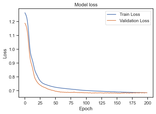
I’ve added two more layers with 32 and 16 nodes, respectively. Now, the model is able to learn the data way faster, while training loss and validation loss are still decreasing and converging. This can be considered a “good model” by the above definition and we could even train it for less epochs.

Conclusion

In summary, autoencoders are valuable tools for dimensionality reduction and data compression. Being a type of artificial neural network, they can be used for learning efficient data encodings in an unsupervised manner. It’s particularly useful for dimensionality reduction, condensing high-dimensional data into a lower-dimensional latent space. This process generates latent variables that, although they may not directly correspond to specific original features, represent combinations of these features. These latent variables can greatly simplify the interpretation of high-dimensional datasets, and can even reveal hidden patterns or structures within the data. While this can be a powerful tool, it’s important to remember that an autoencoder is a machine learning model, and like any other model, it must be validated and fine-tuned. Consider that the steps shown in this post are only a rough guideline and tailored to the Wine dataset. For different datasets and problems you can try out different architectures and hyperparameters and see, which performs best on your validation data.

As always, if you have any questions or suggestions, feel free to leave a comment below or reach out to me on Mastodonꜛ. If you want to learn more about Autoencoders, I recommend the following resources:

• Autoencodersꜛ in the Deep Learning Book by Ian Goodfellow, Yoshua Bengio and Aaron Courville
• Intro to Autoencodersꜛ in the TensorFlow Tutorials
• Building Autoencoders in Kerasꜛ
• Autoencoder Explainedꜛ YouTube video by Brandon Rohrer

The entire code used in this post is also available in this GitHub repositoryꜛ.