Eliminating the middleman: Direct Wasserstein distance computation in WGANs without discriminator

In the previous post, we have seen how we can rewrite a default Generative Adversarial Networks (GAN) to a Wasserstein GAN (WGAN) by changing the loss function of the generator and discriminator. In this post, we explore an alternative approach to implementing WGANs. Contrasting from the standard implementation of WGANs that requires both a generator and discriminator, the method discussed here employs the optimal transport to compute the Wasserstein distance directly between the real and generated data distributions, eliminating the need for a discriminator.

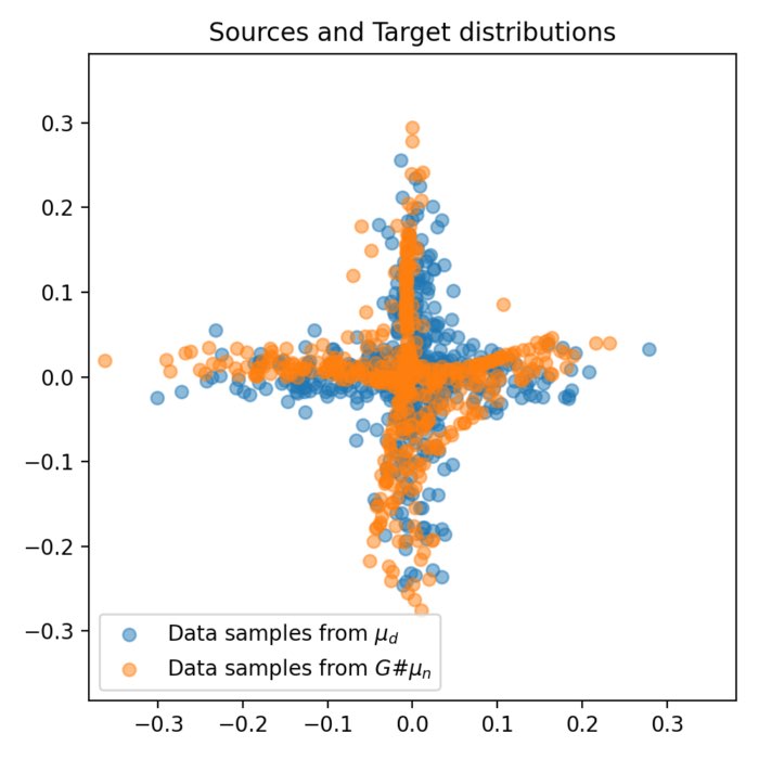
Implementation of the WGAN

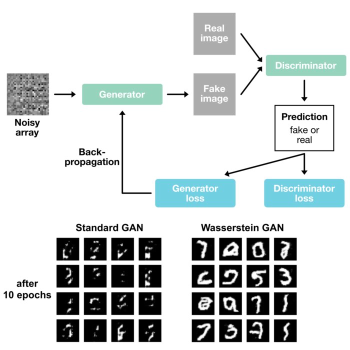
In the usual setup of a Generative Adversarial Network (GAN), we have two components bot a generator and a discriminator. The generator’s task is to generate samples that resemble the true data, while the discriminator’s job is to differentiate between the real and generated data. The generator and discriminator play a kind of game, where the generator is trying to fool the discriminator, and the discriminator is trying not to be fooled.

This dynamic creates a situation where the quality of the generator’s outputs is somewhat dependent on the discriminator’s performance. If the discriminator is too weak, it might not provide meaningful feedback to the generator, resulting in poor quality generated samples. If the discriminator is too strong, it might provide overly harsh feedback, leading to instability in training. This necessitates careful balancing of the training of these two components, often a challenging task.

Wasserstein (WGAN) improves upon the original GAN by using the Wasserstein distance as the loss function, which provides a smooth, differentiable metric that correlates better with the visual quality of generated samples. This model thus has the advantage of overcoming common GAN issues like mode collapse and vanishing gradients. In the previous post we explored, how we can rewrite a default GAN to a Wasserstein GAN by changing the loss function of the generator and discriminator.

On the other hand, a WGAN using the Wasserstein distance more directly fundamentally alters this setup. This variation omits the discriminator network entirely, instead computing the Wasserstein distance directly between the distributions of real and generated data. Here, the cost matrix derived from the optimal transport problem provides an exact measure of the distance between the two distributions, serving as a direct performance metric for the generator. This direct computation offers several advantages. Firstly, it gives a more direct and accurate measure of the generator’s performance since it is based on the exact metric (Wasserstein distance) we’re interested in minimizing. Secondly, it simplifies the training process by removing the need for a discriminator, thereby eliminating the challenge of balancing the training of two adversarial components. Lastly, by directly computing and minimizing the Wasserstein distance, the generator learns to model the true data distribution more robustly and stably. Of course, the efficacy of this approach can be dependent on the specific application and the dimensionality of the data.

Implementation in Python

Let’s see how we can implement the described alternative approach in Python. The code base of the following example comes from this tutorialꜛ of the Python Optimal Transport (POT) library. It uses minibatches to optimize the Wasserstein distance between the real and generated data distributions at each iteration.

For the sake of simplicity, we will use a cross-like distribution as target distribution. The generator will learn to imitate this distribution by generating samples that follow the same distribution. We will use the ot.emd2() function from the POT library to compute the Wasserstein distance between the real and generated data distributions. This function implements the Earth Mover’s Distance (EMD) algorithm, which solves the optimal transport problem and returns the optimal transport cost matrix. This cost matrix provides an exact measure of the distance between the two distributions, serving as a direct performance metric for the generator.

Let’s start by importing the necessary libraries and generating the target distribution:

import numpy as np
import matplotlib.pyplot as plt
import matplotlib.animation as animation
import torch
from torch import nn
import ot

# generate the target distribution:
torch.manual_seed(1)
sigma = 0.1
n_dims = 2
n_features = 2

def get_data(n_samples):
    # set the thickness of the cross:
    thickness = 0.2

    # half samples from vertical line, half from horizontal:
    x_vert = torch.randn(n_samples // 2, 2) * sigma
    x_vert[:, 0] *= thickness  # For vertical line, x-coordinate is always within the range [-thickness/2, thickness/2]

    x_horiz = torch.randn(n_samples // 2, 2) * sigma
    x_horiz[:, 1] *= thickness  # For horizontal line, y-coordinate is always within the range [-thickness/2, thickness/2]

    x = torch.cat((x_vert, x_horiz), 0)
    return x

# plot the distributions
plt.figure(figsize=(5, 5))
x = get_data(500)
plt.figure(1)
plt.scatter(x[:, 0], x[:, 1], label='Data samples from $\mu_d$', alpha=0.5)
plt.title('Data distribution')
plt.legend()

Here is how the target distribution looks like:

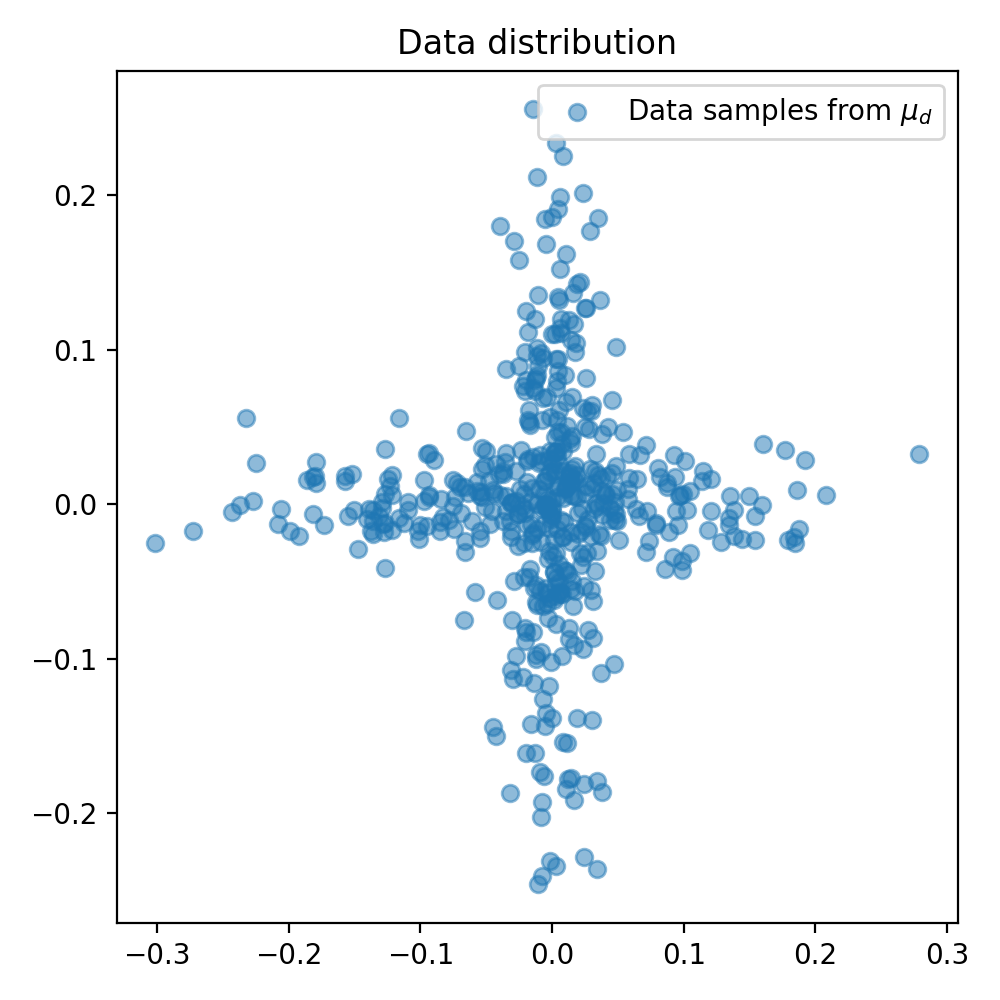The target distribution. The generator will learn to imitate this distribution by generating samples that follow the same distribution.

Next, we define the generator model. The generator is a simple multilayer perceptron (MLP) model, consisting of three fully connected layers and ReLU activation functions. It takes in a random noise vector and outputs a two-dimensional vector, intended to replicate the data distribution

# define the MLP model
class Generator(torch.nn.Module):
    def __init__(self):
        super(Generator, self).__init__()
        self.fc1 = nn.Linear(n_features, 200)
        self.fc2 = nn.Linear(200, 500)
        self.fc3 = nn.Linear(500, n_dims)
        self.relu = torch.nn.ReLU()  # instead of Heaviside step fn

    def forward(self, x):
        output = self.fc1(x)
        output = self.relu(output)  # instead of Heaviside step fn
        output = self.fc2(output)
        output = self.relu(output)
        output = self.fc3(output)
        return output

We train the generator using a gradient descent optimization algorithm, RMSprop. For each training iteration, we:

1. Generate a batch of random noise samples.
2. Generate a corresponding batch of data samples.
3. Feed the noise samples into the generator to obtain a batch of generated samples.
4. Compute the distance matrix between the generated samples and the real data samples.
5. Compute the Wasserstein distance (loss) using ot.emd2(), which calculates the EMD between the two sets of samples.
6. Backpropagate this loss to update the generator’s parameters.

This approach deviates significantly from the typical training regimen of a GAN, where a discriminator model is trained alongside the generator, and their losses are jointly optimized. Here, the generator’s performance is gauged directly on the Wasserstein distance, providing an exact measure of how close the generator’s distribution is to the target distribution.

G = Generator()
optimizer = torch.optim.RMSprop(G.parameters(), lr=0.00019, eps=1e-5)

# number of iteration and size of the batches:
n_iter = 200  # set to 200 for doc build but 1000 is better ;)
size_batch = 500

# generate static samples to see their trajectory along training:
n_visu = 100
xnvisu = torch.randn(n_visu, n_features)
xvisu = torch.zeros(n_iter, n_visu, n_dims)

ab = torch.ones(size_batch) / size_batch
losses = []

for i in range(n_iter):
    # generate noise samples:
    xn = torch.randn(size_batch, n_features)

    # generate data samples:
    xd,_ = get_data(size_batch)

    # generate sample along iterations:
    xvisu[i, :, :] = G(xnvisu).detach()

    # generate samples and compte distance matrix:
    xg = G(xn)
    M = ot.dist(xg, xd)

    loss = ot.emd2(ab, ab, M)
    losses.append(float(loss.detach()))

    if i % 10 == 0:
        print("Iter: {:3d}, loss={}".format(i, losses[-1]))

    loss.backward()
    optimizer.step()

    del M

The rest of the code is dedicated to visualizing the results. For the sake of brevity, I will not show these parts here, but you can find the full code in the GitHub repository mentioned at the end of this post.

Here are the results of the generator’s training:

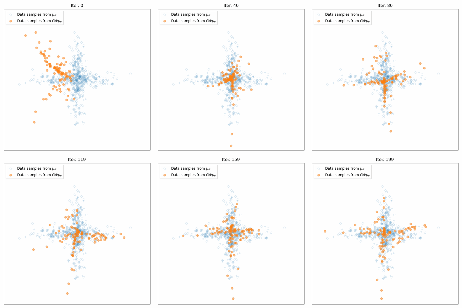
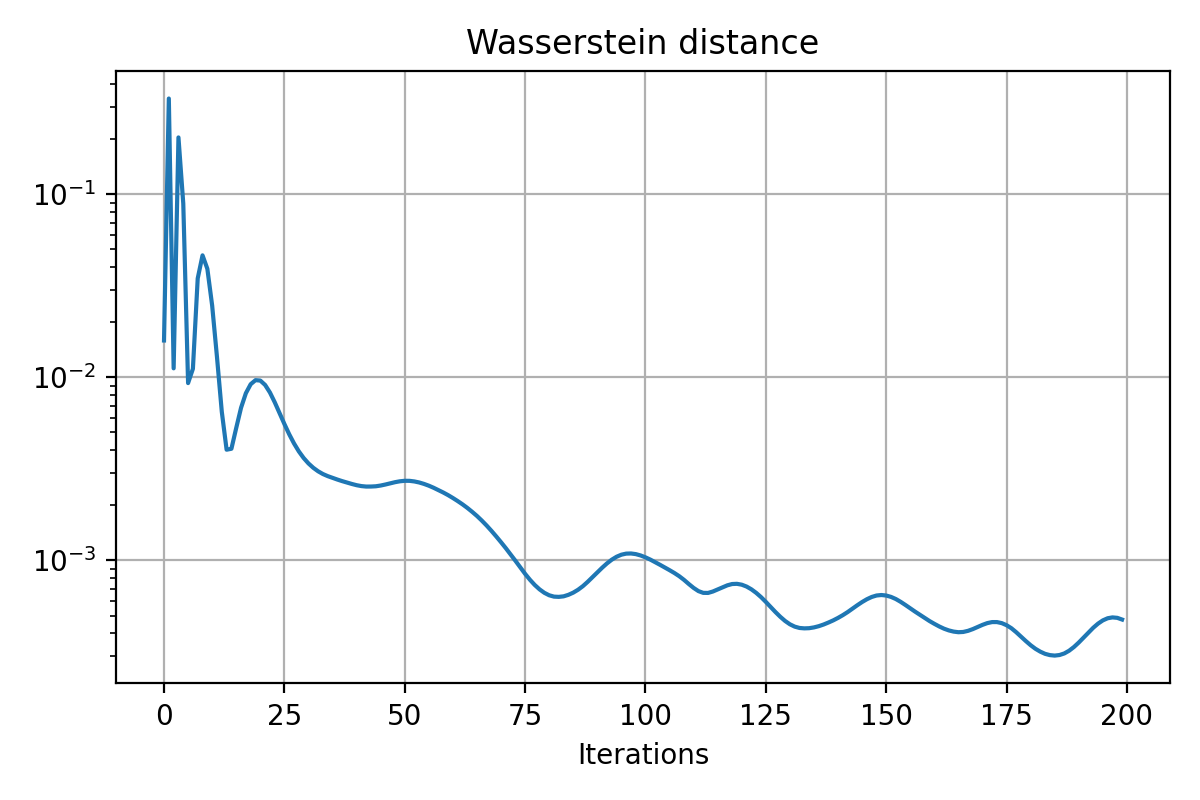
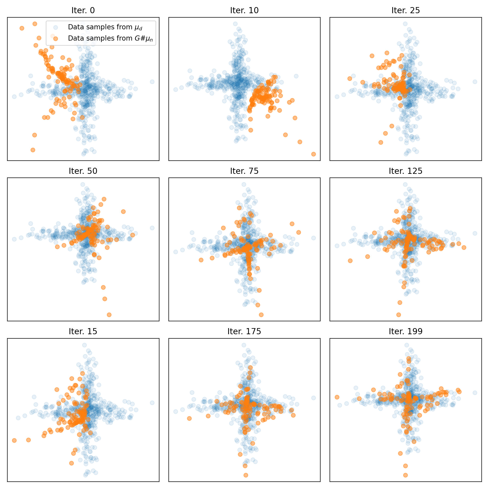Results of the generator’s training on the cross-like distribution. Top: Animation of the generator’s training. Middle: The Wasserstein distance between the real and generated data distributions as a function of iteration. Bottom: Some snapshots of the generated samples. The generator successfully learns to mimic the cross-like distribution of the real data.

The performance of the generator is evaluated by monitoring the Wasserstein distance along the iterations. As expected, we see this distance decreasing over time, indicating that the generated distribution is progressively converging to the real data distribution. Furthermore, the snapshots of the generated samples show that the generator successfully learns to mimic the cross-like distribution of the real data.

Since I fell in love with the animation of the generator’s training, I also run the script on two further target distributions: a sinusoidal distribution,

def get_data(n_samples):
    # Generates a 2D dataset of samples forming a sine wave with noise.
    
    x = torch.linspace(-np.pi, np.pi, n_samples).view(-1, 1)
    y = torch.sin(x) + sigma * torch.randn(n_samples, 1)
    data = torch.cat((x, y), 1)
    data_sample_name = 'sine'
    return data, data_sample_name

and a circular distribution,

def get_data(n_samples):
    # Generates a 2D dataset of samples forming a circle with noise.
    
    c = torch.rand(size=(n_samples, 1))
    angle = c * 2 * np.pi
    x = torch.cat((torch.cos(angle), torch.sin(angle)), 1)
    x += torch.randn(n_samples, 2) * sigma
    data_sample_name = 'circle'
    return x, data_sample_name

The latter is from the original POT documentation tutorial. Here are the training results:

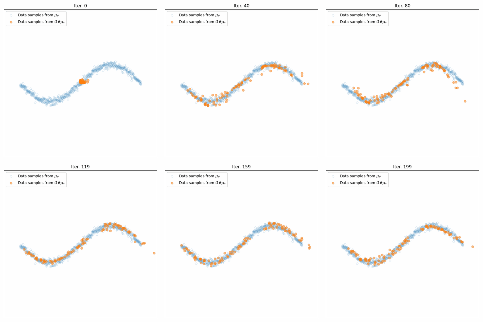
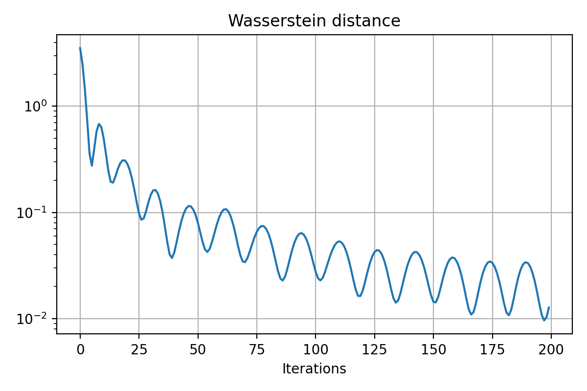
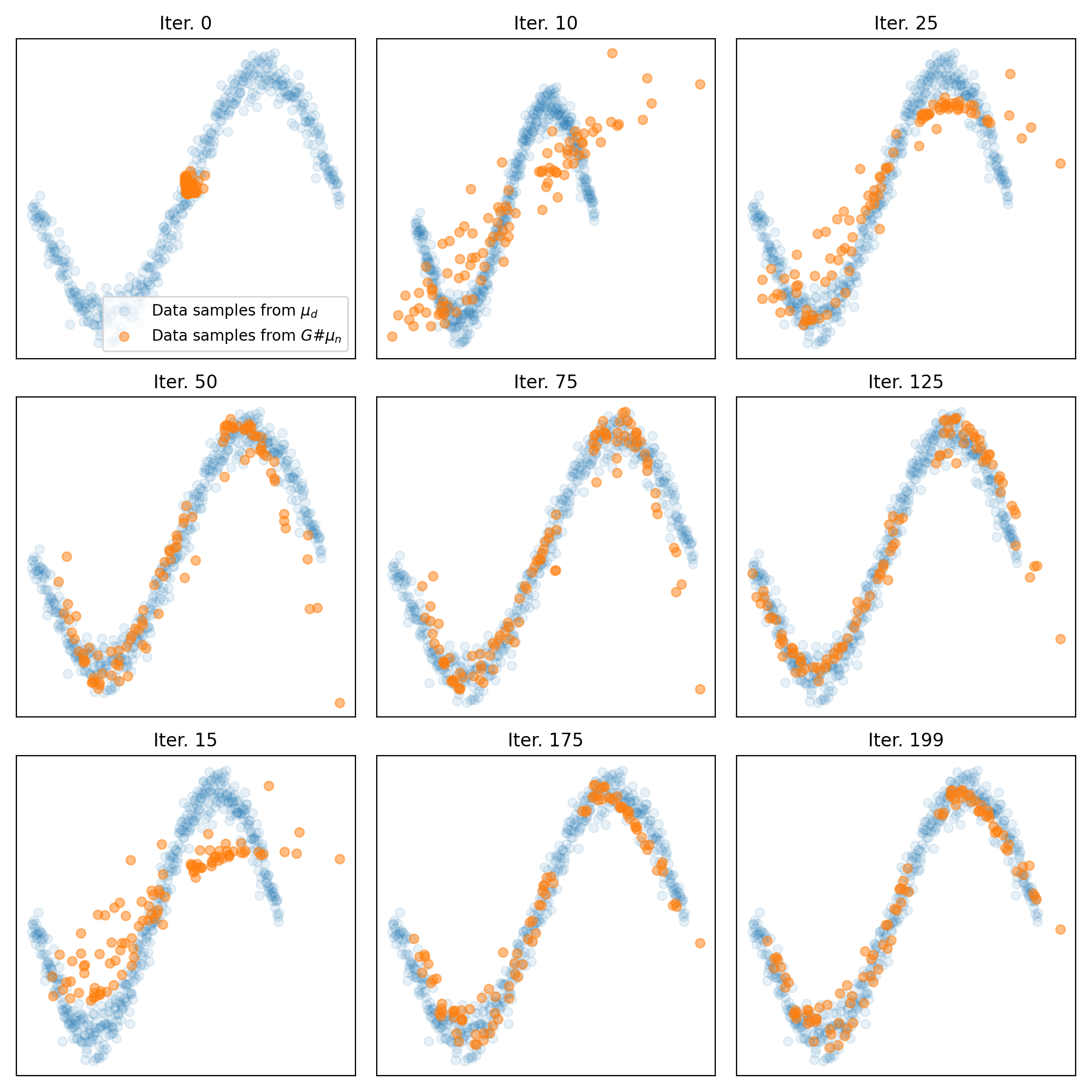Results for training on a sinusoidal distribution. Top: Animation of the generator’s training. Middle: The Wasserstein distance between the real and generated data distributions. Bottom: Snapshots of the generated samples.

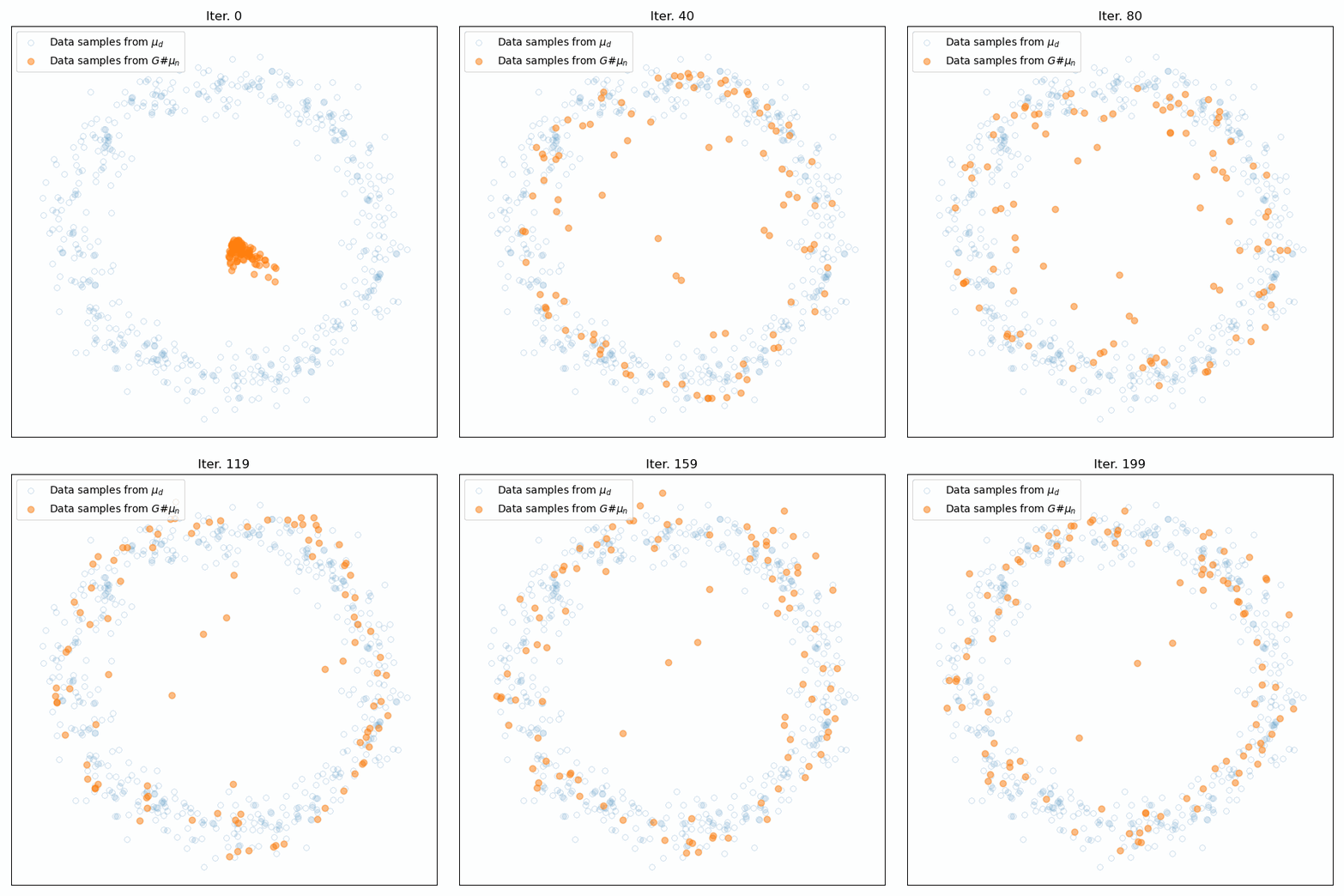
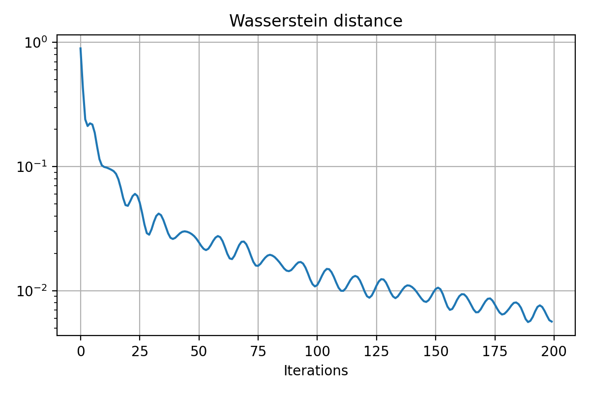
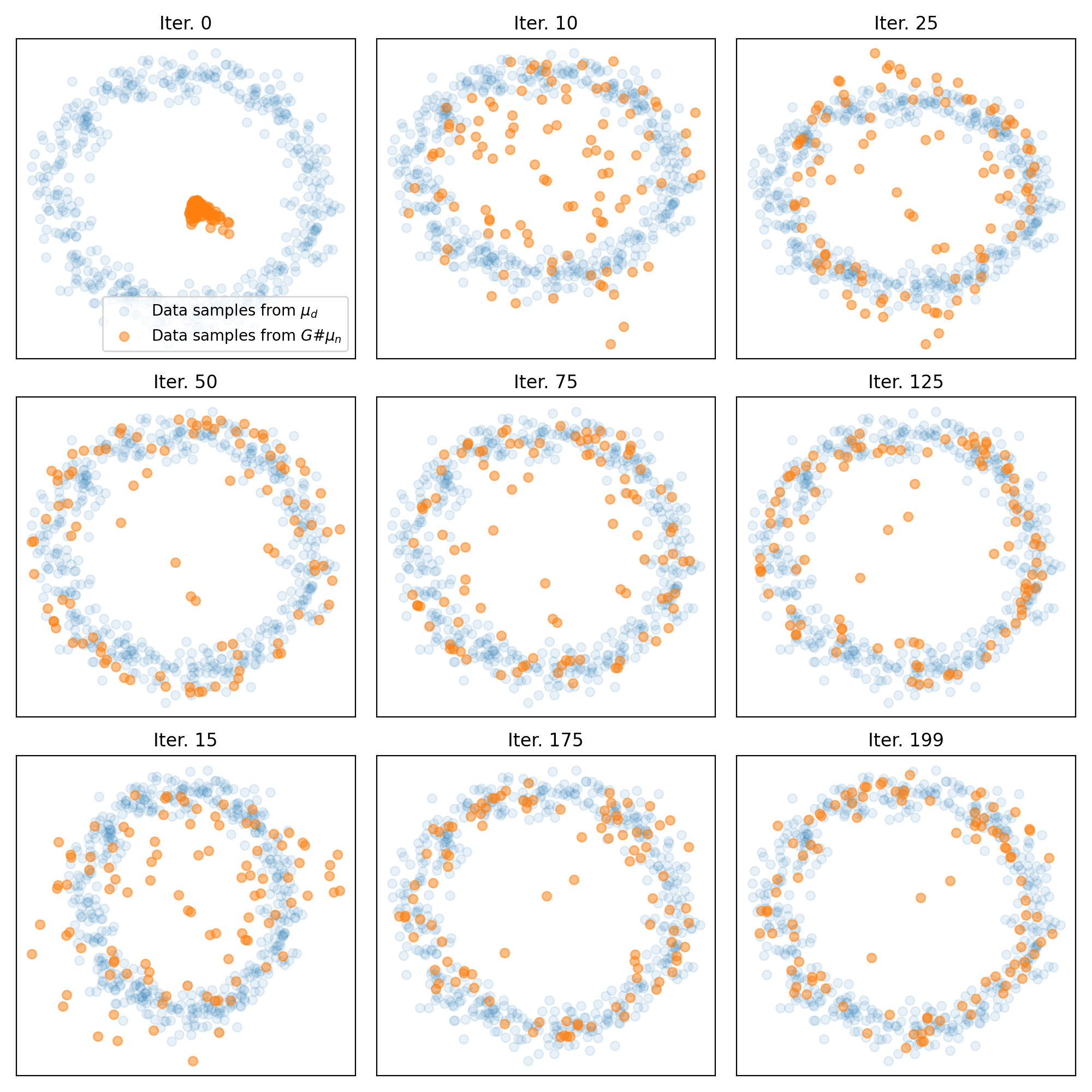Results for training on a circular distribution. Top: Animation of the generator’s training. Middle: The Wasserstein distance between the real and generated data distributions. Bottom: Snapshots of the generated samples.

Conclusion

The advantage of the demonstrated approach lies in its direct computation of the Wasserstein distance using optimal transport methods, resulting in a more straightforward and intuitive understanding of how the generator improves over time. It abstains from the need for a discriminator network and the challenge of balancing its training with the generator’s. Consequently, it results in a stable and robust generative model that directly optimizes the very metric (Wasserstein distance) that WGANs were designed to improve.

In conclusion, I think employing the ot.emd2() function to compute the Wasserstein distance provides an insightful perspective on the WGAN framework. By focusing on the Wasserstein distance directly, it allows for an intuitive understanding of the generator’s performance and mitigates several challenges associated with traditional GAN training. Despite the evident differences in the approaches, both offer valuable insights into the functioning and benefits of Wasserstein GANs, and their choice is influenced by the problem specifics and computational resources.

The code used in this post is available in this GitHub repositoryꜛ.

If you have any questions or suggestions, feel free to leave a comment below.