Excurse: Improving the learning in ANN

12 minute read

In this chapter, we briefly explore techniques and strategies to improve the training of artificial neural networks (ANNs). These methods address several key challenges in neural network training, particularly overfitting and underfitting, and help ensure that the network generalizes well to unseen data.

Effective ANN training requires tuning a variety of parameters and applying techniques to balance learning speed, generalization, and accuracy. Each section below discusses a specific technique or concept, explaining its purpose, application, and effect on network training.

Loss curve monitoring

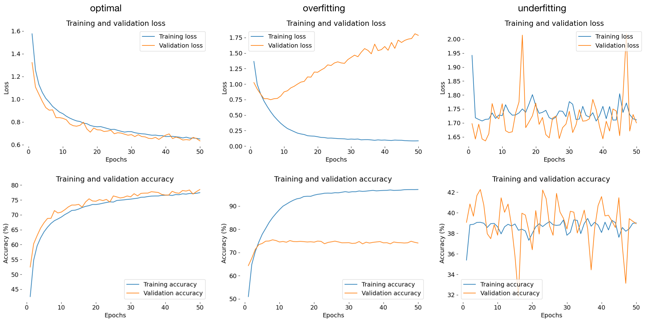
Loss curves provide a graphical representation of the model’s performance over time. By plotting training and validation loss across epochs, we can monitor learning trends and detect overfitting:

Converging loss: A steady decrease in training and validation loss indicates successful learning.
Diverging loss: If validation loss increases while training loss decreases, it suggests overfitting.
Underfitting: If both losses are high, the model may need more epochs or tuning.

Overview of training and validation loss (top row) and accuracy curves (bottom row) for optimal (left), overfitting (middle), and underfitting (right) scenarios. Optimal training: Training and validation losses decrease smoothly and converge, with validation loss slightly higher than training loss, indicating a good generalization. Both training and validation accuracies increase over time and stabilize close to each other, demonstrating a balanced fit. Overfitting: The training loss continually decreases to near zero, while the validation loss begins to rise after initially decreasing, indicating that the model is memorizing the training data but failing to generalize. Training accuracy approaches 100%, while validation accuracy plateaus at a lower level, showing a clear gap that indicates overfitting. Underfitting: In Training and validation losses fluctuate without clear improvement, indicating that the model fails to learn significant patterns from the data. Training and validation accuracies remain low and inconsistent throughout, suggesting the model’s capacity is insufficient to capture the underlying structure of the data.

Loss curves help diagnose issues early and guide hyperparameter adjustments.

Hyperparameters

Hyperparameters are the settings chosen before training a model, not learned from data. In the following, we discuss key hyperparameters and their impact on training.

Learning rate

The learning rate controls the step size in updating weights and thus the speed at which the model updates weights during training. Setting an optimal learning rate is crucial:

high learning rate: Faster convergence but risks overshooting the minimum of the loss function, which can lead to unstable training.
low learning rate: Slower convergence but can lead to more precise weight updates. However, it may get stuck in local minima and require many epochs to converge.

Adaptive learning rate scheduling

Learning rate schedulers adjust the learning rate over time, helping to balance speed and precision. Common scheduling techniques include:

Step decay: Reduces the learning rate by a fixed factor after a set number of epochs.
Exponential decay: Reduces the learning rate continuously by a fixed factor.
Cyclical learning rate: Alternates between a high and low learning rate, which can help the model escape shallow local minima.
Reduce on plateau: Reduces the learning rate when the model’s performance stops improving, commonly used in conjunction with validation loss monitoring.

Learning rate warm-up

Learning rate warm-up gradually increases the learning rate at the beginning of training, allowing the model to explore the loss landscape more effectively before settling into a stable learning rate. This helps with training stability in early epochs.

Number of epochs

An epoch is a full pass through the entire training dataset. Selecting the right number of epochs is important:

Underfitting: Too few epochs may lead to underfitting, where the model hasn’t learned enough from the data.
Overfitting: Too many epochs may lead to overfitting, where the model starts memorizing the training data instead of learning generalizable patterns.

Early stopping

Early stopping is a technique that monitors validation loss and halts training if it stops improving after a set number of epochs (patience). This technique prevents overfitting and saves computation time by stopping training as soon as the model starts to overfit.

Batch size

The batch size dictates the number of samples processed before updating model parameters. Smaller batch sizes can provide more stable updates, while larger sizes may speed up training. We will further discuss batch and mini-batch training below.

Regularization strength

The regularization strength controls the penalty applied to prevent overfitting. Regularization techniques like L2 and L1 regularization add penalties to the loss function to discourage complex models. We will explore this further below.

Hyperparameter optimization

Hyperparameter tuning or optimization is the process of finding optimal values for these parameters to enhance the network’s performance. Here are some common techniques:

Grid search: A method of systematically trying different combinations of hyperparameters to find the best configuration. Although computationally expensive, it provides an exhaustive search.
Random search: Instead of trying every combination, random search samples from the hyperparameter space, reducing computation time with comparable effectiveness.
Bayesian optimization: An advanced technique that models the hyperparameter tuning process as a probabilistic optimization problem. It’s especially useful for tuning complex models.
Hyperband: A bandit-based optimization algorithm that allocates resources efficiently by pruning poorly performing configurations early.
Population-based training: A method that evolves a population of hyperparameters over time, allowing for efficient exploration of the hyperparameter space.

Batch size and mini-batch training

The batch size is the number of training samples processed before the model’s parameters are updated. Training can be performed in several modes based on batch size:

Batch gradient descent: Uses the entire dataset for each update, which provides stable updates but is computationally intensive and memory demanding.
Stochastic gradient descent (SGD): Uses one sample per update, introducing noise that can help escape local minima but may lead to unstable convergence.
Mini-Batch gradient descent: Uses a small subset of samples (mini-batch) per update, combining the stability of batch gradient descent with the speed of SGD.

Mini-batch sizes of 32, 64, or 128 are common choices, as they provide a balance between memory usage, computational efficiency, and stable learning.

Weight initialization

Weight initialization is crucial for training deep networks, as improper initialization can lead to vanishing or exploding gradients. Proper weight initialization helps with stable gradient flow through layers.

Common initialization techniques are:

Xavier (Glorot) Initialization: Suitable for sigmoid and tanh activations. It keeps the variance of weights similar across layers, promoting stable gradients.
\[W \sim \mathcal{U}\left(-\frac{\sqrt{6}}{\sqrt{n_{\text{in}} + n_{\text{out}}}}, \frac{\sqrt{6}}{\sqrt{n_{\text{in}} + n_{\text{out}}}}\right)\]
He Initialization: Designed for ReLU activations, it scales weights based on the number of input neurons to prevent vanishing gradients.
\[W \sim \mathcal{N}\left(0, \frac{2}{n_{\text{in}}}\right)\]

These methods ensure that activations don’t vanish or explode as they propagate through layers, leading to smoother training.

Regularization techniques

Regularization techniques add penalties to the loss function, discouraging overly complex models and improving generalization by reducing overfitting.

L2 Regularization (Weight Decay)

L2 regularization penalizes large weights by adding the sum of squared weights to the loss function. This drives weights closer to zero, making the model simpler and less prone to overfitting:

\[L_{\text{total}} = L_{\text{data}} + \lambda \sum w^2\]

where $\lambda$ is a hyperparameter controlling the regularization strength.

L1 Regularization

L1 regularization penalizes the absolute values of weights, promoting sparsity by driving some weights to zero:

\[L_{\text{total}} = L_{\text{data}} + \lambda \sum |w|\]

L1 regularization is often used in applications where sparse solutions are desired.

Dropout

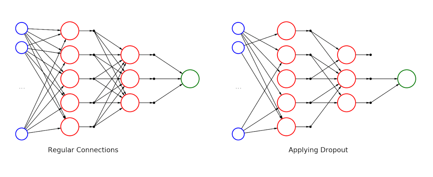
Dropout is a form of regularization where a random fraction of neurons is deactivated during each forward pass, reducing co-dependencies among neurons. This prevents overfitting by forcing the network to rely on various subsets of neurons, making it more resilient. Dropout rates of 0.2–0.5 are common for hidden layers.

On the left is a fully connected neural network with two hidden layers. On the right is the same network after applying dropout. Source: Wikimedia Commonsꜛ (license: CC BY-SA 4.0)

Optimizer

The optimizer is the algorithm that updates model parameters based on the gradients computed during backpropagation. Each optimizer has strengths and weaknesses, and the choice depends on the specific task and model architecture. Common optimizers include:

Stochastic gradient descent (SGD)

SGD updates parameters for each mini-batch, which is computationally efficient and suitable for large datasets. Momentum is often added to SGD to maintain direction in parameter space and speed up convergence.

Adam

Adam (Adaptive Moment Estimation) is a widely used optimizer that combines the benefits of momentum and RMSprop. It adapts learning rates based on the first and second moments of gradients, enabling efficient training with minimal tuning.

RMSprop

RMSprop (Root Mean Square Propagation) maintains a moving average of squared gradients, which smooths parameter updates and reduces oscillations. It’s effective for models with complex error surfaces.

Batch normalization

Batch Normalization normalizes inputs to each layer, stabilizing and accelerating training. It reduces internal covariate shift (changes in the distribution of inputs to each layer during training), which makes the network less sensitive to the initial weights and learning rate.

For each mini-batch, batch normalization standardizes activations by subtracting the batch mean and dividing by the batch standard deviation:

\[\hat{x} = \frac{x - \mu}{\sqrt{\sigma^2 + \epsilon}}\]

where $\mu$ and $\sigma^2$ are the batch mean and variance, and $\epsilon$ is a small constant to avoid division by zero.

Batch normalization reduces the need for dropout, simplifies hyperparameter tuning, and improves convergence.

Cross-validation

Cross-validation splits the dataset into multiple subsets (folds), providing multiple train-validation splits to better assess model robustness. K-fold cross-validation is popular, where the data is divided into $K$ subsets, and each subset serves as the validation set once, while the rest serve as the training set.

Cross-validation mitigates overfitting by ensuring that model evaluation does not depend on a single train-validation split. This technique provides a more robust estimate of the model’s generalization ability.

Data augmentation

Data augmentation generates additional training data by applying transformations like rotations, flips, and scaling. This technique increases dataset diversity, improving model generalization by making it less likely to overfit.

Examples of common data augmentations:

Image augmentations: Flipping, cropping, rotation, and scaling.
Noise injection: Adding noise to input data, particularly in audio and signal processing.

Data augmentation is especially effective in image recognition, where it can increase effective training set size and help the model learn invariances.

Model complexity

Model complexity or architecture tuning involves selecting the appropriate number of layers, neurons, and activation functions for the task. A model that is too simple may underfit, while a model that is too complex may overfit.

Summary

Improving the training of ANNs requires a careful balance of techniques to ensure effective learning and generalization. In summary:

Loss curve monitoring: Observing trends in training and validation loss.
Hyperparameter tuning: Optimizing learning rate, epochs, and batch size for balanced training.
Weight initialization: Techniques like Xavier and He initialization to stabilize gradient flow.
Regularization: L2, L1, and dropout to prevent overfitting.
Optimizer selection: Choosing the right optimizer based on task requirements.
Batch normalization: Standardizing activations to improve training stability.
Cross-validation: Ensuring robustness by evaluating on multiple train-validation splits.
Data augmentation: Expanding the training set with transformations to improve generalization.
Model complexity: Tuning the architecture to balance underfitting and overfitting.

Each method contributes uniquely to stabilizing training, enhancing generalization, and accelerating convergence. Proper application of these techniques allows neural networks to learn complex patterns while avoiding common pitfalls like overfitting and underfitting.

Python examples

In the following Python example, we demonstrate how to implement a simple neural network (fully connected (dense) neural network) for image classification using PyTorch. The model includes dropout, batch normalization, and custom weight initialization to improve learning and generalization. We train the model on the MNIST dataset and evaluate its performance on a test set.

We begin by importing the necessary libraries:

import numpy as np
import matplotlib.pyplot as plt

import torch
import torch.nn as nn
import torch.optim as optim
import torchvision.transforms as transforms
import torchvision.datasets as datasets
from torch.utils.data import DataLoader, random_split

Next, we define the hyperparameters:

# hyperparameters:
learning_rate = 0.001   # change the learning
batch_size = 64         # change the batch size
epochs = 10             # change the number of epochs
weight_decay = 1e-4     # choose a L2 regularization strength, here: weight decay

We then define the dataset and data augmentation transformations:

# dataset and data augmentation
transform = transforms.Compose([
    transforms.RandomRotation(10),          # data augmentation
    transforms.RandomHorizontalFlip(),      # data augmentation
    transforms.ToTensor(),
    transforms.Normalize((0.5,), (0.5,))    # normalize to [-1, 1]
])

dataset = datasets.MNIST(root='./data', train=True, transform=transform, download=True)
train_size = int(0.8 * len(dataset))
val_size = len(dataset) - train_size
train_data, val_data = random_split(dataset, [train_size, val_size])

test_data = datasets.MNIST(root='./data', train=False, transform=transform)
train_loader = DataLoader(train_data, batch_size=batch_size, shuffle=True)
val_loader = DataLoader(val_data, batch_size=batch_size)
test_loader = DataLoader(test_data, batch_size=batch_size)

Next, we define the neural network model with dropout, batch normalization, and custom weight initialization:

class SimpleNN(nn.Module):
    def __init__(self):
        super(SimpleNN, self).__init__()
        self.fc1 = nn.Linear(28*28, 512)
        self.bn1 = nn.BatchNorm1d(512)   # batch normalization
        self.dropout1 = nn.Dropout(0.3)  # dropout for regularization
        self.fc2 = nn.Linear(512, 256)
        self.bn2 = nn.BatchNorm1d(256)
        self.dropout2 = nn.Dropout(0.3)
        self.fc3 = nn.Linear(256, 10)

        # Initialize weights
        self._init_weights()

    def _init_weights(self):
        # He initialization (good for ReLU activations)
        nn.init.kaiming_normal_(self.fc1.weight, nonlinearity='relu')
        nn.init.kaiming_normal_(self.fc2.weight, nonlinearity='relu')
        nn.init.xavier_normal_(self.fc3.weight)

    def forward(self, x):
        x = x.view(-1, 28*28)
        x = torch.relu(self.bn1(self.fc1(x)))
        x = self.dropout1(x)
        x = torch.relu(self.bn2(self.fc2(x)))
        x = self.dropout2(x)
        x = self.fc3(x)
        return x

We then instantiate the model, define the loss function, and select the optimizer:

# instantiate model, loss function, and optimizer:
device= torch.device('mps')
#device = torch.device('cuda' if torch.cuda.is_available() else 'cpu')
model = SimpleNN().to(device)
criterion = nn.CrossEntropyLoss()
optimizer = optim.Adam(model.parameters(), lr=learning_rate, weight_decay=weight_decay)

We train the model with early stopping and track training and validation losses:

train_losses = []
val_losses = []
patience = 3
early_stop_count = 0
best_val_loss = float('inf')

for epoch in range(epochs):
    model.train()
    epoch_train_loss = 0
    for images, labels in train_loader:
        images, labels = images.to(device), labels.to(device)
        
        optimizer.zero_grad()
        outputs = model(images)
        loss = criterion(outputs, labels)
        loss.backward()
        optimizer.step()
        
        epoch_train_loss += loss.item()

    train_loss = epoch_train_loss / len(train_loader)
    train_losses.append(train_loss)

    # validation: (no gradient calculation needed)
    model.eval()
    epoch_val_loss = 0
    with torch.no_grad():
        for images, labels in val_loader:
            images, labels = images.to(device), labels.to(device)
            outputs = model(images)
            loss = criterion(outputs, labels)
            epoch_val_loss += loss.item()

    val_loss = epoch_val_loss / len(val_loader)
    val_losses.append(val_loss)
    
    print(f'Epoch {epoch+1}/{epochs}, Train Loss: {train_loss:.4f}, Val Loss: {val_loss:.4f}')

    # early stopping check:
    if val_loss < best_val_loss:
        best_val_loss = val_loss
        early_stop_count = 0
    else:
        early_stop_count += 1
        if early_stop_count >= patience:
            print("Early stopping triggered.")
            break

Finally, we evaluate the model on the test set and visualize some sample predictions

# plot training and validation losses:
plt.figure(figsize=(8, 5))
plt.plot(train_losses, label='Training Loss')
plt.plot(val_losses, label='Validation Loss')
plt.xlabel('Epoch')
plt.ylabel('Loss')
plt.title('Training and Validation Loss over Epochs')
plt.legend()
plt.grid(True)
plt.show()

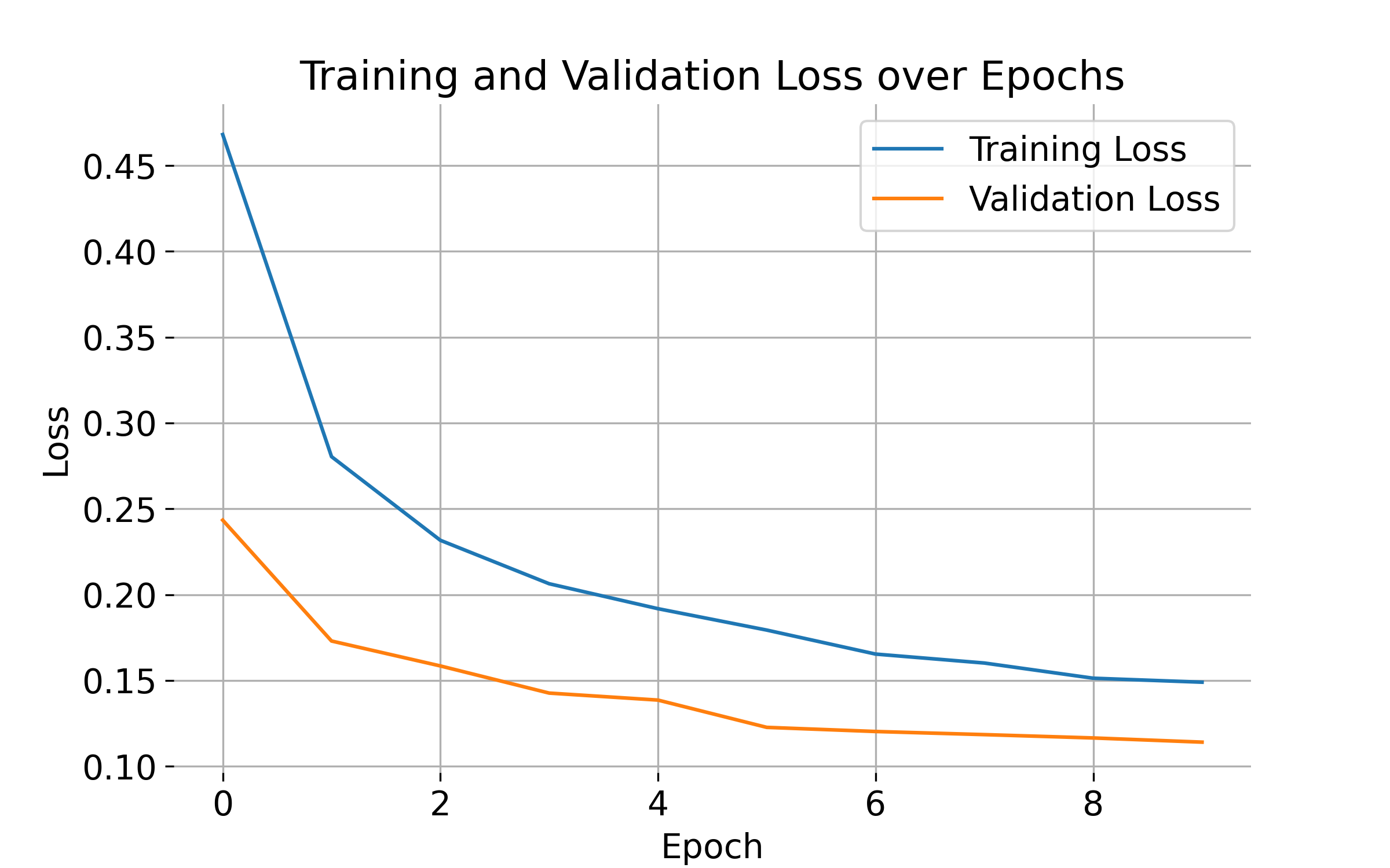
Training and validation loss over epochs. The plot shows the training and validation loss decreasing over epochs, indicating that the model is learning from the data and generalizing well. Monitoring the loss helps track the model’s progress and identify potential issues like overfitting or underfitting.

# testing and prediction visualization:
model.eval()
correct = 0
total = 0
predictions = []
images_list = []

with torch.no_grad():
    for images, labels in test_loader:
        images, labels = images.to(device), labels.to(device)
        outputs = model(images)
        _, predicted = torch.max(outputs.data, 1)
        total += labels.size(0)
        correct += (predicted == labels).sum().item()

        # collect a few images and predictions for visualization:
        if len(images_list) < 10:
            images_list.extend(images[:5])
            predictions.extend(predicted[:5])

print(f'Test Accuracy: {100 * correct / total:.2f}%')

# plot some sample predictions:
plt.figure(figsize=(10, 5))
for i, (img, pred) in enumerate(zip(images_list, predictions)):
    plt.subplot(2, 5, i + 1)
    plt.imshow(img.cpu().numpy().squeeze(), cmap='gray')
    plt.title(f"Pred: {pred.item()}")
    plt.axis('off')
plt.show()

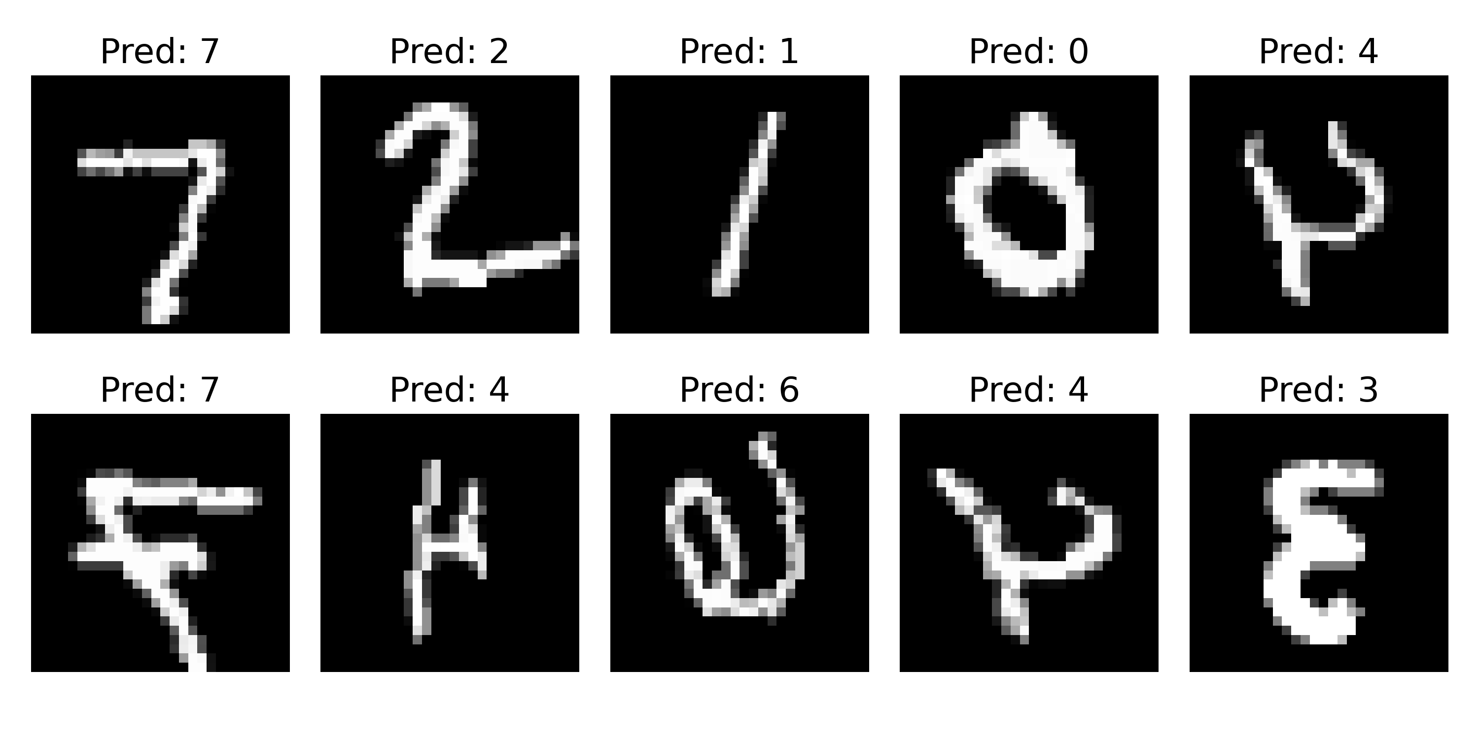
Predictions of our model on a few test images. The model correctly identifies the digits in the images, demonstrating its ability to generalize to unseen data. Visualization helps verify the model’s performance and identify potential errors.