Autoencoders (AE)

Autoencoders (AEs) are a class of neural networks used for unsupervised learning tasks. Their main purpose is to learn a lower-dimensional representation of input data by training the network to reconstruct the input from its compressed form. This compressed, or latent, representation captures the most important features of the data and can be used for tasks like dimensionality reduction, anomaly detection, and even generative modeling. Autoencoders leverage the network’s ability to encode complex, high-dimensional data into a more compact form while retaining essential characteristics.

Structure of Autoencoders

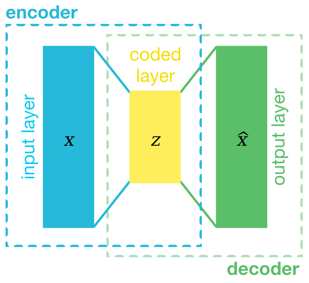
An autoencoder is a type of neural network that consists of three main components:

• the encoder part, which compresses the input data into a lower-dimensional latent space,
• the latent space (or coded space), which captures the essential features of the input data, and
• the decoder part, which reconstructs the original input from the latent representation.

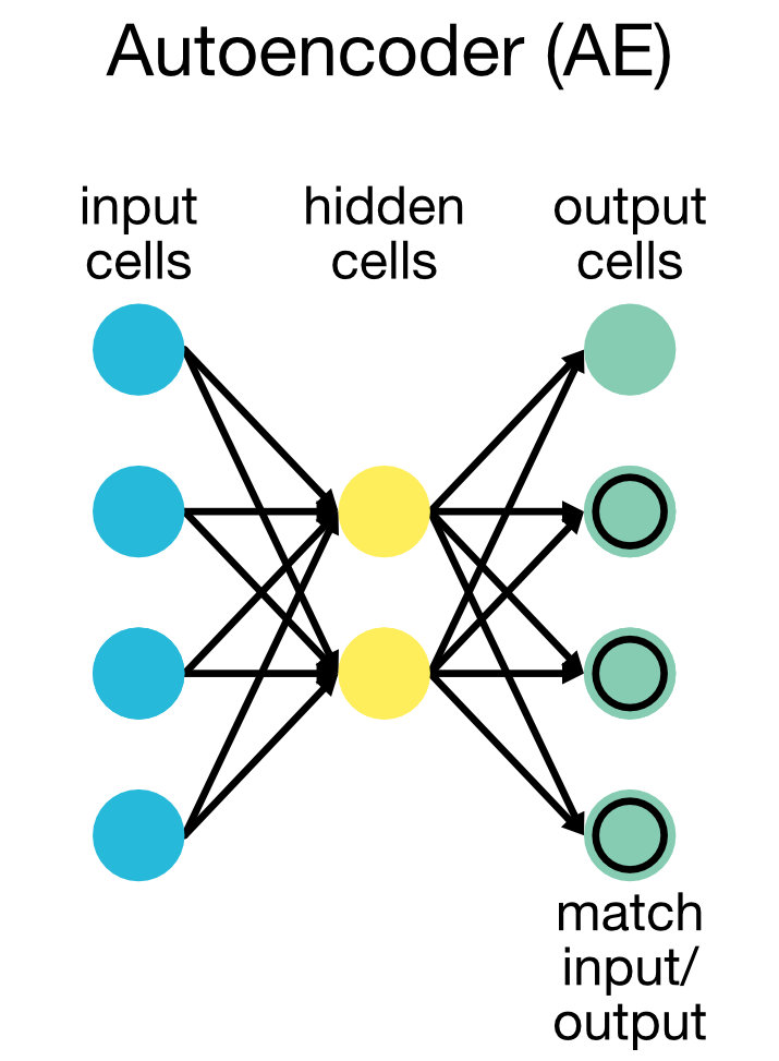
In its simplest form, an autoencoder consist of three layers: an input layer, a hidden layer (latent space), and an output layer:

Schematic representation of an autoencoder in its simplest form: 3 layers, consisting of an input layer, a latent space, and an output layer.

The architecture outlined above is a stark simplification and the actual structure of an autoencoder is indeed more complex. In practice, autoencoders can have multiple layers in the encoder and decoder, making them deep autoencoders:

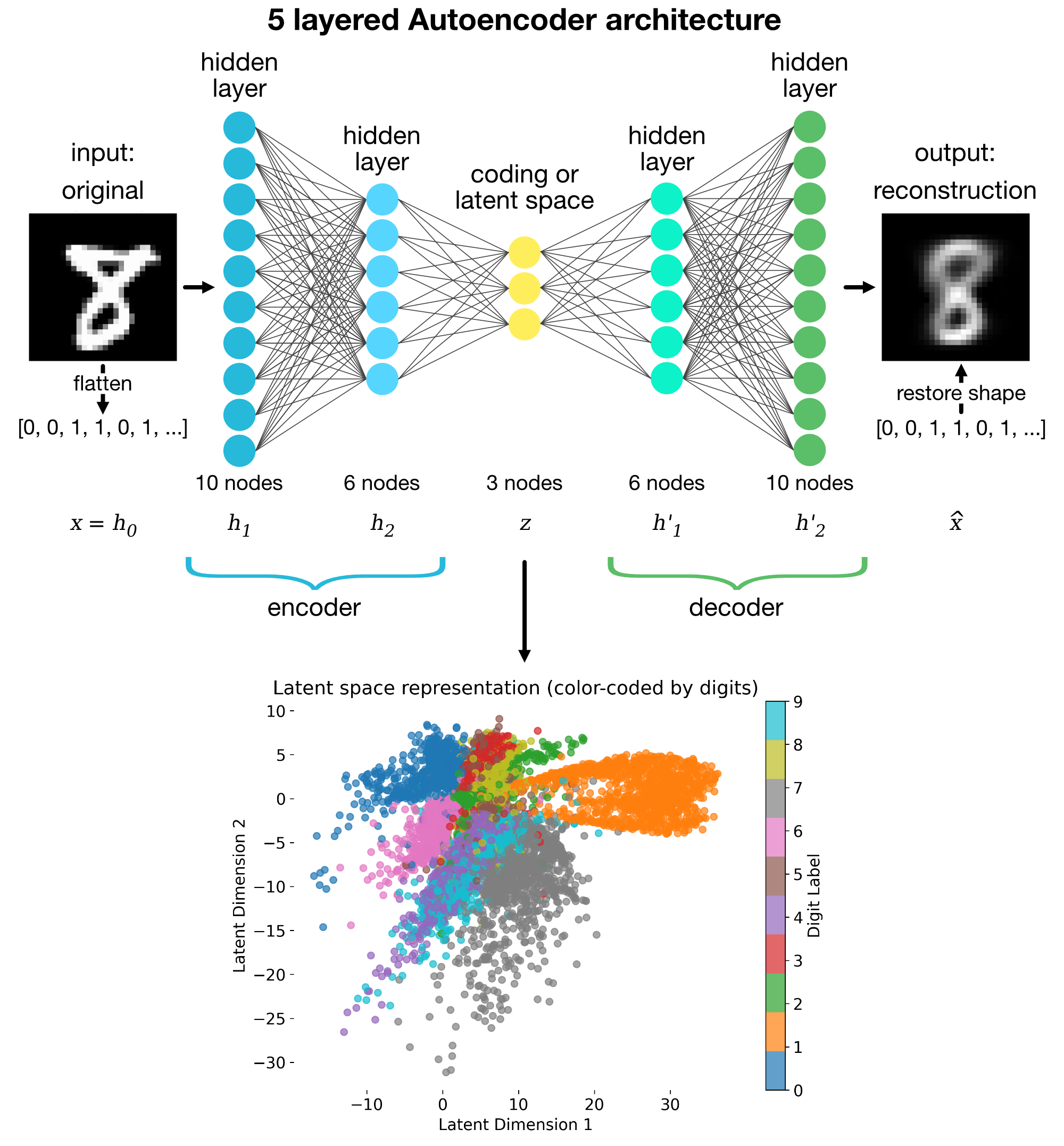Architecture of an 5-layered autoencoder with encoder, latent space, and decoder parts.

The number of layers and the size of the latent space can be adjusted based on the complexity of the data and the desired level of compression. Here is a general description of each component:

Encoder

The encoder reduces the dimensionality of the input data by applying a series of transformations across multiple layers. For an autoencoder with $N$ total layers in the encoder, the input data $\mathbf{x}$ is successively transformed from one layer to the next, until it reaches the latent space representation, $\mathbf{z}$. Each transformation applies weights, biases, and an activation function to the data.

For each layer $i$, where $i = 1, 2, …, N$, the transformation from the previous layer’s output (or input data in the case of the first layer) can be expressed as:

\[\mathbf{h}_i = \sigma(\mathbf{W}_i \mathbf{h}_{i-1} + \mathbf{b}_i)\]

where:

• $\mathbf{h}_0 = \mathbf{x}$ is the input data,
• $\mathbf{h}_i$ is the output of the $i$-th layer (also called the hidden layer),
• $\mathbf{W}_i$ and $\mathbf{b}_i$ are the weights and biases for layer $i$,
• $\sigma$ is the activation function (e.g., ReLU, sigmoid),
• $N$ is the total number of layers in the encoder.

Each node in the network applies an activation function $\sigma$ to the weighted sum of its inputs to introduce non-linearity into the model. Common activation functions include ReLU (Rectified Linear Unit), sigmoid, and tanh. The choice of activation function can impact the network’s ability to learn complex patterns and avoid issues like the vanishing gradient problem.

The final hidden layer of the encoder produces the latent space representation $\mathbf{z}$:

\[\mathbf{z} = \mathbf{h}_N = \sigma(\mathbf{W}_N \mathbf{h}_{N-1} + \mathbf{b}_N)\]

Thus, the input data is progressively compressed across multiple layers into the lower-dimensional latent space $\mathbf{z}$, which captures the most important features of the input.

Latent Space (or Coding Layer)

The latent space, $\mathbf{z}$, is the compressed form of the input data. It typically has far fewer dimensions than the original input, but it retains the key information necessary for reconstructing the input. This compression is crucial for tasks like dimensionality reduction, feature extraction, and data denoising, as it filters out less relevant details while retaining the most significant patterns.

Decoder

The decoder takes the latent space representation $\mathbf{z}$ and reconstructs the original input data by applying another series of transformations, reversing the process of the encoder. The decoder is structured symmetrically to the encoder, with $N$ layers.

For each layer $j$ in the decoder, where $j = 1, 2, …, N$, the latent representation $\mathbf{z}$ is successively transformed back into the original input space:

\[\mathbf{h}_j' = \sigma(\mathbf{W}_j' \mathbf{h}_{j-1}' + \mathbf{b}_j')\]

where:

• $\mathbf{h}_0’ = \mathbf{z}$ is the input to the decoder (the latent space),
• $\mathbf{h}_j’$ is the output of the $j$-th layer of the decoder,
• $\mathbf{W}_j’$ and $\mathbf{b}_j’$ are the weights and biases for the $j$-th layer of the decoder.

The output of the final layer of the decoder is the reconstruction of the original input $\mathbf{\hat{x}}$:

\[\mathbf{\hat{x}} = \sigma(\mathbf{W}_N' \mathbf{h}_{N-1}' + \mathbf{b}_N')\]

The objective of the decoder is to produce an output $\mathbf{\hat{x}}$ that closely matches the original input $\mathbf{x}$. To achieve this, the network minimizes the reconstruction loss during training, which measures the difference between the original data $\mathbf{x}$ and the reconstructed output $\mathbf{\hat{x}}$.

Loss function of Autoencoders

The performance of an autoencoder is evaluated by its ability to minimize the reconstruction error between the original input $\mathbf{x}$ and the reconstructed output $\mathbf{\hat{x}}$. The loss function typically depends on the type of data:

Reconstruction loss for continuous data:

The most common loss function for continuous data is the Mean Squared Error (MSE), which measures the squared differences between the original and reconstructed data:

\[L(\mathbf{x}, \hat{\mathbf{x}}) = \frac{1}{n} \sum_{i=1}^{n} ||\mathbf{x}_i - \hat{\mathbf{x}}_i||^2\]

Reconstruction loss for binary data:

For binary or probabilistic data, the Binary Cross-Entropy Loss is often used:

\[L(\mathbf{x}, \mathbf{\hat{x}}) =\] \[-\sum_{i=1}^{n} \left( x_i \log(\hat{x}_i) + (1 - x_i) \log(1 - \hat{x}_i) \right)\]

The overall objective of the autoencoder is to minimize the reconstruction error across the entire dataset:

\[\min_{\theta, \phi} \frac{1}{n} \sum_{i=1}^{n} L(\mathbf{x}_i, \mathbf{\hat{x}}_i)\]

where $n$ represents the number of data points, and $L(\mathbf{x}_i, \mathbf{\hat{x}}_i)$ is the loss function for the $i$-th data point. This ensures that the autoencoder learns an effective compression of the data while minimizing the reconstruction error.

The minimization of the reconstruction loss is achieved through backpropagation and gradient descent optimization, where the network’s weights and biases are updated iteratively to reduce the loss. Here’s how the training process works:

1. Forward pass:

The input $\mathbf{x}$ is fed into the encoder, which transforms it layer by layer into the latent space representation $\mathbf{z}$. $\mathbf{z}$ is then passed through the decoder, which reconstructs the input as $\hat{\mathbf{x}}$, the predicted output.

2. Reconstruction loss:

The difference between the original input $\mathbf{x}$ and the reconstructed output $\hat{\mathbf{x}}$ is measured using a loss function $L(\mathbf{x}, \hat{\mathbf{x}})$. The loss quantifies how well the autoencoder is able to reconstruct the original input data.

3. Backpropagation:

Once the loss is computed, backpropagation is used to minimize the loss. Backpropagation works by:

1. Calculating the gradient of the loss with respect to each of the parameters in the network (weights and biases in both the encoder and decoder).
2. Updating the parameters using an optimization algorithm such as stochastic gradient descent (SGD) or one of its variants like Adam. The parameter update for each weight $w$ is given by:

\[w_{\text{new}} = w_{\text{old}} - \eta \cdot \frac{\partial L}{\partial w}\]

where $\eta$ is the learning rate, and $\frac{\partial L}{\partial w}$ is the gradient of the loss with respect to the weight $w$.

4. Parameter update:

This process of updating the weights continues iteratively over many epochs (passes through the entire training dataset), gradually reducing the reconstruction error. The encoder learns to compress the data in a way that retains important information, while the decoder learns to reconstruct the data from this compressed form as accurately as possible.

5. Repeat:

The forward pass, loss computation, backpropagation, and weight update steps are repeated for each batch of input data over multiple training epochs until the model converges (i.e., the reconstruction loss stabilizes and reaches a minimum) or until a predefined stopping criterion is met.

Types of Autoencoders

There are several types of autoencoders, each designed for different tasks:

1. Vanilla Autoencoder: This is the simplest form of autoencoder with fully connected layers. Both the encoder and decoder are composed of dense layers.
2. Convolutional Autoencoder: Designed for image data, convolutional autoencoders use convolutional layers in both the encoder and decoder to capture spatial hierarchies in the data.
3. Sparse Autoencoder: This type of autoencoder includes a regularization term to encourage sparsity in the latent representation, where only a few neurons are active at a time. It enforces a form of feature selection, making the learned features more interpretable.
4. Denoising Autoencoder: In this variant, the autoencoder is trained to reconstruct the original data from a noisy version of the input. This makes the model robust to noise, which is especially useful in image or signal processing.
5. Variational Autoencoder (VAE): A VAE is a probabilistic model where the encoder maps the input data to a distribution (mean and variance) rather than a fixed vector. VAEs are often used in generative modeling, allowing the generation of new data samples from the learned latent space.

Encoder and decoder architectures

The encoder typically consists of several layers that progressively reduce the input data’s dimensionality. Non-linear activations such as ReLU or sigmoid are applied to introduce flexibility into the model. The final layer outputs the latent representation $\mathbf{z}$.

Example:

\[\mathbf{x} \rightarrow \text{Dense Layer} \rightarrow \text{ReLU} \rightarrow \dots \rightarrow \mathbf{z}\]

The decoder mirrors the encoder’s architecture. It takes the latent representation $\mathbf{z}$ and progressively expands it back to the original dimensionality of the input data.

Example:

\[\mathbf{z} \rightarrow \text{Dense Layer} \rightarrow \text{ReLU} \rightarrow \dots \rightarrow \mathbf{\hat{x}}\]

Applications of Autoencoders

• Dimensionality reduction: Autoencoders compress data into a lower-dimensional latent space while preserving essential information, functioning similarly to PCA but with the added ability to capture non-linear relationships.
• Anomaly detection: By reconstructing the input data, autoencoders can identify anomalies based on high reconstruction errors, as anomalous data points are typically difficult to reconstruct.
• Denoising: Denoising autoencoders remove noise from corrupted data, learning robust representations of the original data.
• Data compression: Autoencoders can be used to compress data for efficient storage or transmission, reducing redundancy while retaining key information.
• Generative models: VAEs are used to generate new samples by sampling from the latent space, making them useful for tasks such as image synthesis.

Advantages and limitations of autoencoders

Advantages:

• Non-linear representations: Unlike linear methods like PCA, autoencoders can model non-linear relationships in the data.
• Customizable architectures: The number of layers, layer sizes, and other architectural features can be tailored to the specific problem and dataset.
• Unsupervised learning: Autoencoders do not require labeled data, making them useful for unsupervised learning tasks like feature extraction.

Limitations:

• Data dependency: Autoencoders are typically limited to reconstructing data similar to the training set and may struggle with generalizing to completely new data.
• Training complexity: Training neural networks requires careful tuning of hyperparameters and can be computationally intensive.
• Interpretability: The latent space representations learned by autoencoders may not always be interpretable compared to simpler, linear methods.

Conclusion

Autoencoders are versatile tools for learning compact representations of data. By leveraging neural networks, they offer powerful techniques for dimensionality reduction, anomaly detection, and generative modeling. However, their success depends on careful architectural design and tuning, and they may not always generalize well to new data.

Python example

In this example, we demonstrate how to implement an autoencoder using PyTorch to compress and reconstruct images from the MNIST dataset. The MNIST dataset consists of 28x28 grayscale images of handwritten digits (0-9). We define a simple autoencoder architecture with fully connected layers and train it on the dataset. Finally, we visualize the reconstructed images and the latent space representation.

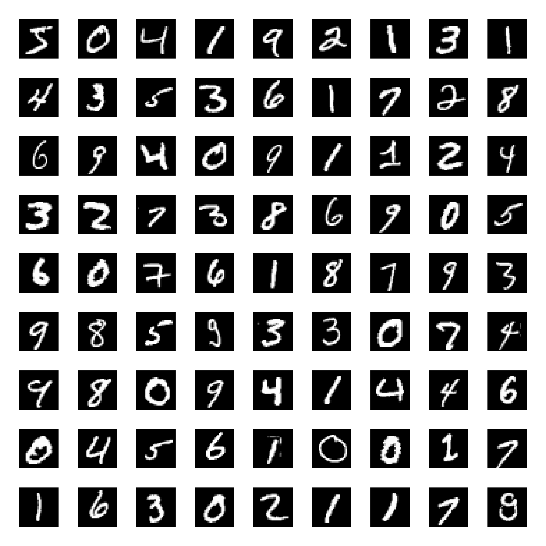Samples from the MNIST dataset, which consists of over 60,000 grayscale images (28x28 pixels) of handwritten digits (0-9).

Let’s begin by importing the necessary libraries and preparing the dataset:

import os
import numpy as np
import matplotlib.pyplot as plt

import torch
import torch.nn as nn
import torch.optim as optim
from torchvision import datasets, transforms

# for reproducibility:
torch.manual_seed(1)

The MNIST dataset consists of 60,000 training images and 10,000 test images of handwritten digits (0–9). The dataset is already pre-split into a training set and a test set by default when downloaded from torchvision.datasets:

# download and prepare the MNIST dataset:
transform = transforms.Compose([transforms.ToTensor(), transforms.Normalize((0.5,), (0.5,))])

train_data = datasets.MNIST(root='./data', train=True, download=True, transform=transform)
test_data  = datasets.MNIST(root='./data', train=False, download=True, transform=transform)

train_loader = torch.utils.data.DataLoader(train_data, batch_size=256, shuffle=True)
test_loader  = torch.utils.data.DataLoader(test_data, batch_size=256, shuffle=True)

Each image is converted into a tensor and normalized using the transforms.Compose function. transforms.Normalize((0.5,), (0.5,)) normalizes the image pixel values to be in the range [-1, 1], with a mean of 0.5 and standard deviation of 0.5. This helps with training by standardizing the inputs.

After loading the datasets, they are passed to the PyTorch DataLoader (torch.utils.data.DataLoader) to create iterable batches of data.

Next, we define our Autoencoder model. The model consists of an encoder and a decoder, each defined as a sequence of fully connected layers with ReLU activation functions. The encoder compresses the input image (28x28 pixels) into a 2-dimensional latent space, while the decoder reconstructs the image back to its original size.

# autoencoder definition:
class Autoencoder(nn.Module):
    def __init__(self):
        super(Autoencoder, self).__init__()
        self.encoder = nn.Sequential(
            nn.Linear(28*28, 128),
            nn.ReLU(),
            nn.Linear(128, 64),
            nn.ReLU(),
            nn.Linear(64, 12),
            nn.ReLU(),
            nn.Linear(12, 2)  # 2 dimensions for the latent space
        )
        self.decoder = nn.Sequential(
            nn.Linear(2, 12),
            nn.ReLU(),
            nn.Linear(12, 64),
            nn.ReLU(),
            nn.Linear(64, 128),
            nn.ReLU(),
            nn.Linear(128, 28*28),
            nn.Tanh()
        )

    def forward(self, x):
        encoded = self.encoder(x)
        decoded = self.decoder(encoded)
        return encoded, decoded

# instantiate the model, loss function, and optimizer:
model = Autoencoder()

# on macOS, move the model to the MPS device:
device = torch.device('mps')
model = model.to(device)

We need to define the loss function and optimizer for training the autoencoder. We use the Mean Squared Error (MSE) loss to measure the difference between the input and the reconstructed output. The Adam optimizer is used to update the model parameters during training:

learning_rate = 1e-3
criterion = nn.MSELoss()
optimizer = optim.Adam(model.parameters(), lr=learning_rate)

Now, we are ready to train the autoencoder on the MNIST dataset. We iterate over the training data for a specified number of epochs, compute the loss, and update the model parameters using backpropagation:

# training the autoencoder:
num_epochs = 20
train_losses = []
val_losses = []

for epoch in range(num_epochs):
    model.train()
    running_loss = 0
    for images, _ in train_loader:
        images = images.view(images.size(0), -1).to(device)
        optimizer.zero_grad()
        encoded, decoded = model(images)
        loss = criterion(decoded, images)
        loss.backward()
        optimizer.step()
        running_loss += loss.item()
    train_losses.append(running_loss / len(train_loader))
    
    # Validation
    model.eval()
    val_loss = 0
    with torch.no_grad():
        for images, _ in test_loader:
            images = images.view(images.size(0), -1).to(device)
            encoded, decoded = model(images)
            loss = criterion(decoded, images)
            val_loss += loss.item()
    val_losses.append(val_loss / len(test_loader))
    
    print(f"Epoch {epoch+1}, Train Loss: {train_losses[-1]:.4f}, Val Loss: {val_losses[-1]:.4f}")

After training the autoencoder, we visualize the loss curves and the reconstructed images to evaluate the model’s performance:

# plot loss curves:
plt.figure(figsize=(6, 4))
plt.plot(train_losses, label='Training Loss')
plt.plot(val_losses, label='Validation Loss')
plt.title('Loss Curves')
plt.xlabel('Epochs')
plt.ylabel('MSE Loss')
plt.legend()
plt.show()

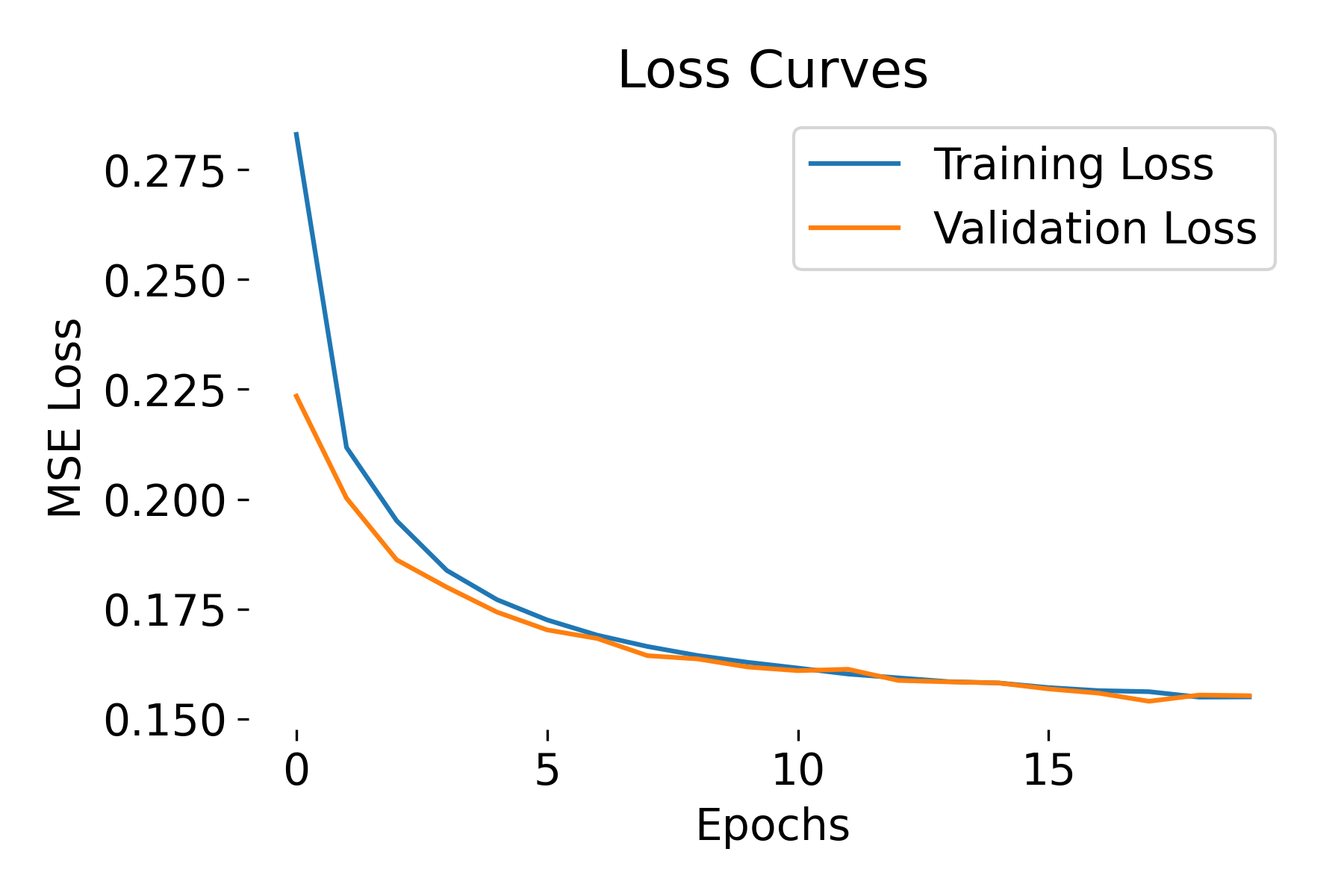Loss curves during training of the Autoencoder.

To visualize the reconstructed images, we select a batch of test images, pass them through the trained autoencoder, and plot the original and reconstructed images side by side:

# select a batch of test images:
model.eval()
with torch.no_grad():
    images, _ = next(iter(test_loader))  # get a batch of test images
    images = images.view(images.size(0), -1).to(device)
    encoded, decoded = model(images)
    decoded = decoded.view(decoded.size(0), 28, 28).cpu()  # reshape the decoded image to 28x28

# plot the first image and its reconstruction:
n = 1  # you can change this to visualize a different image in the batch
plt.figure(figsize=(6, 3))
# plot original image:
plt.subplot(1, 2, 1)
plt.imshow(images[n].view(28, 28).cpu().numpy(), cmap='gray')
plt.title('Original Image')
plt.axis('off')

# plot reconstructed image:
plt.subplot(1, 2, 2)
plt.imshow(decoded[n].cpu().numpy(), cmap='gray')
plt.title('Reconstructed Image')
plt.axis('off')
plt.show()

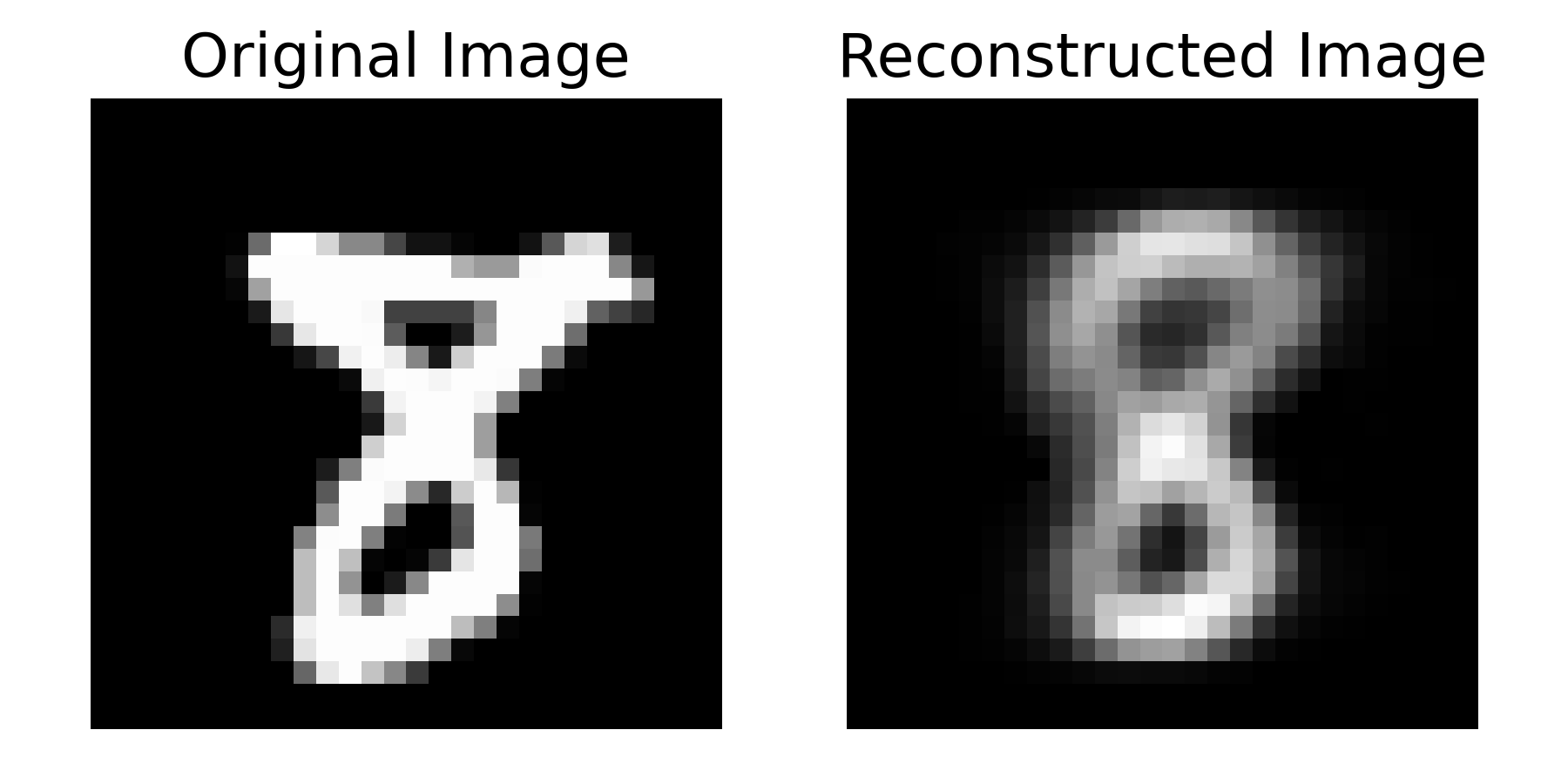Sample original image (left, “8”) and reconstructed image (right).

Why do we switch the model to evaluation mode and disable gradient computation during visualization?

After training, we switch the model into evaluation mode using model.eval() and disable gradient computations with torch.no_grad(). This reduces memory and computation overhead, which is useful when we’re just encoding data without needing backpropagation. This step ensures we’re focusing on inference without extra overhead from gradients.

Storing the latent space at every step during training can increase memory usage and complexity since training involves many iterations (forward/backward passes) where gradients are computed. Thus, we decided to store the latent space representation only after training is complete.

Let’s have a look at how the Autoencoder compresses the MNIST images into a 2-dimensional latent space:

# visualizing the latent space:
model.eval()
latents = []
labels = []

# we need to disable gradient computation for this step:
with torch.no_grad():
    for images, lbls in test_loader:
        images = images.view(images.size(0), -1).to(device)
        encoded, _ = model(images)
        latents.append(encoded.cpu().numpy())
        labels.append(lbls.cpu().numpy())

latents = np.concatenate(latents)
labels = np.concatenate(labels)

# plot the latent space, color-coded by digit labels
plt.figure(figsize=(8, 6))
scatter = plt.scatter(latents[:, 0], latents[:, 1], c=labels, cmap='tab10', alpha=0.7)
plt.colorbar(scatter, label='Digit Label')
plt.title('Latent space representation (color-coded by digits)')
plt.xlabel('Latent Dimension 1')
plt.ylabel('Latent Dimension 2')
plt.show()

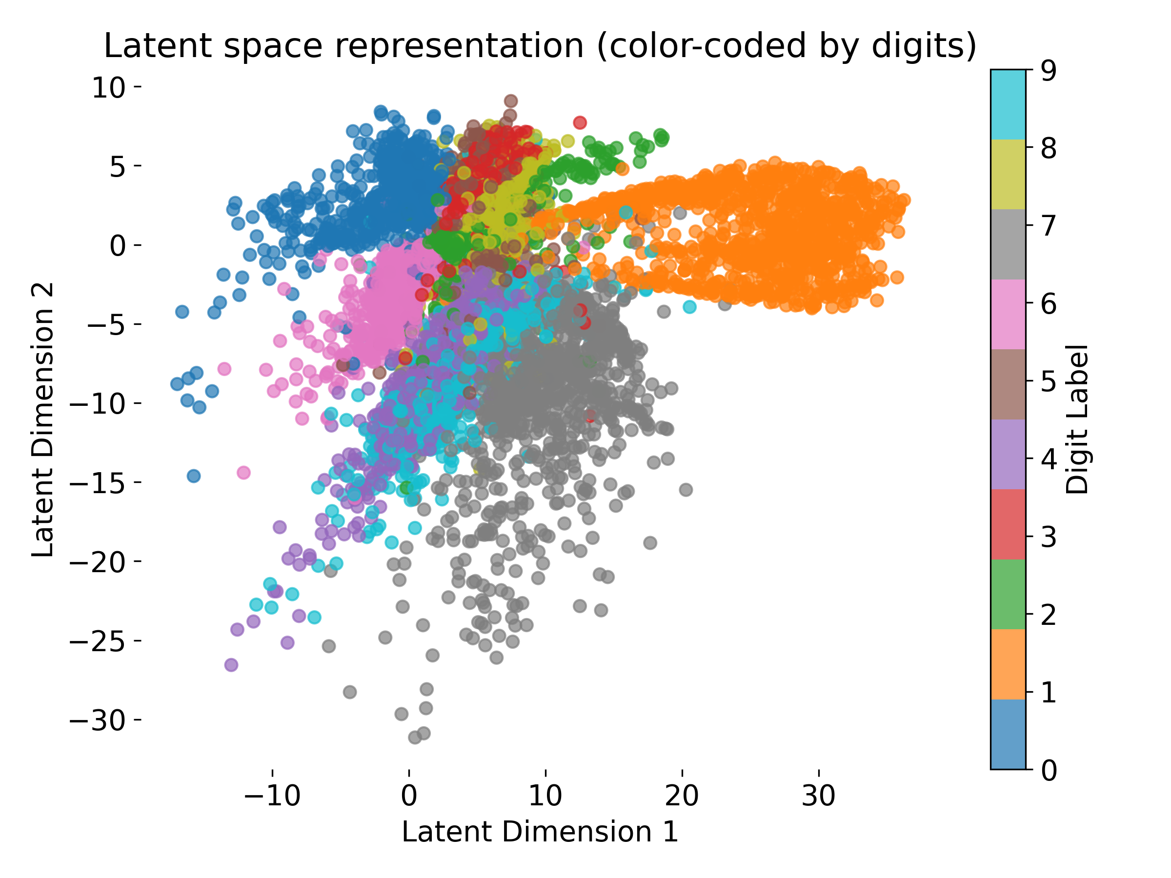Latent space representation of MNIST digits color-coded by digit labels.

In case, you are not satisfied with the results, you can further fine-tune the model by adjusting the :

• architecture: add more layers, change the number of neurons in each layer, or experiment with different activation functions and regularization techniques
• hyperparameters: change the learning rate, batch size, etc.
• training duration: train the model for more epochs or with a larger dataset

Exercise

We have two exercises on Autoencoders. The first exercise will guide you through implementing a simple autoencoder using PyTorch on neural data that we have analyzed in the previous two exercises (PCA and clustering). The second exercise will extend the autoencoder to also embed the behavior data into the latent space of a second neural dataset. This will allow you to explore the potential of autoencoders for integrating multiple data modalities.

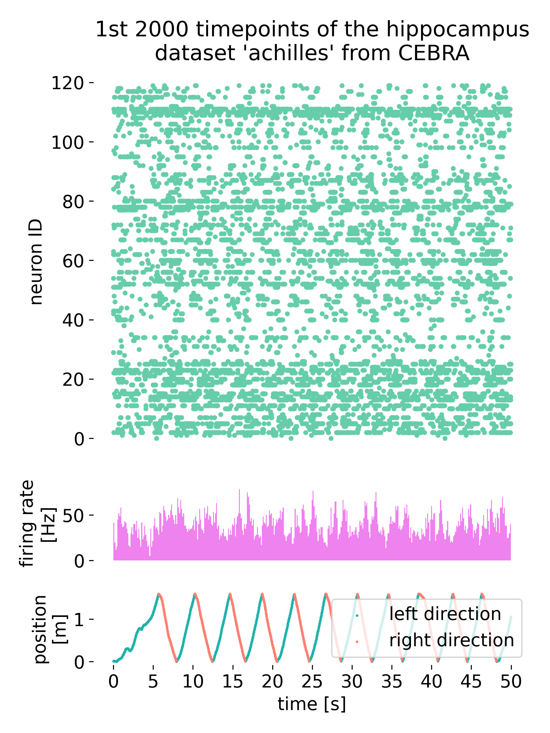The second neural data used in the exercise. Shown are the responses of neurons to the behavior performed by the mouse. Upper plot shows the spike rasters of hippocampal neurons, the middle plot shows the histogram of the firing rates of all neurons, and the lower plot shows the behavior performed by the mouse (location).

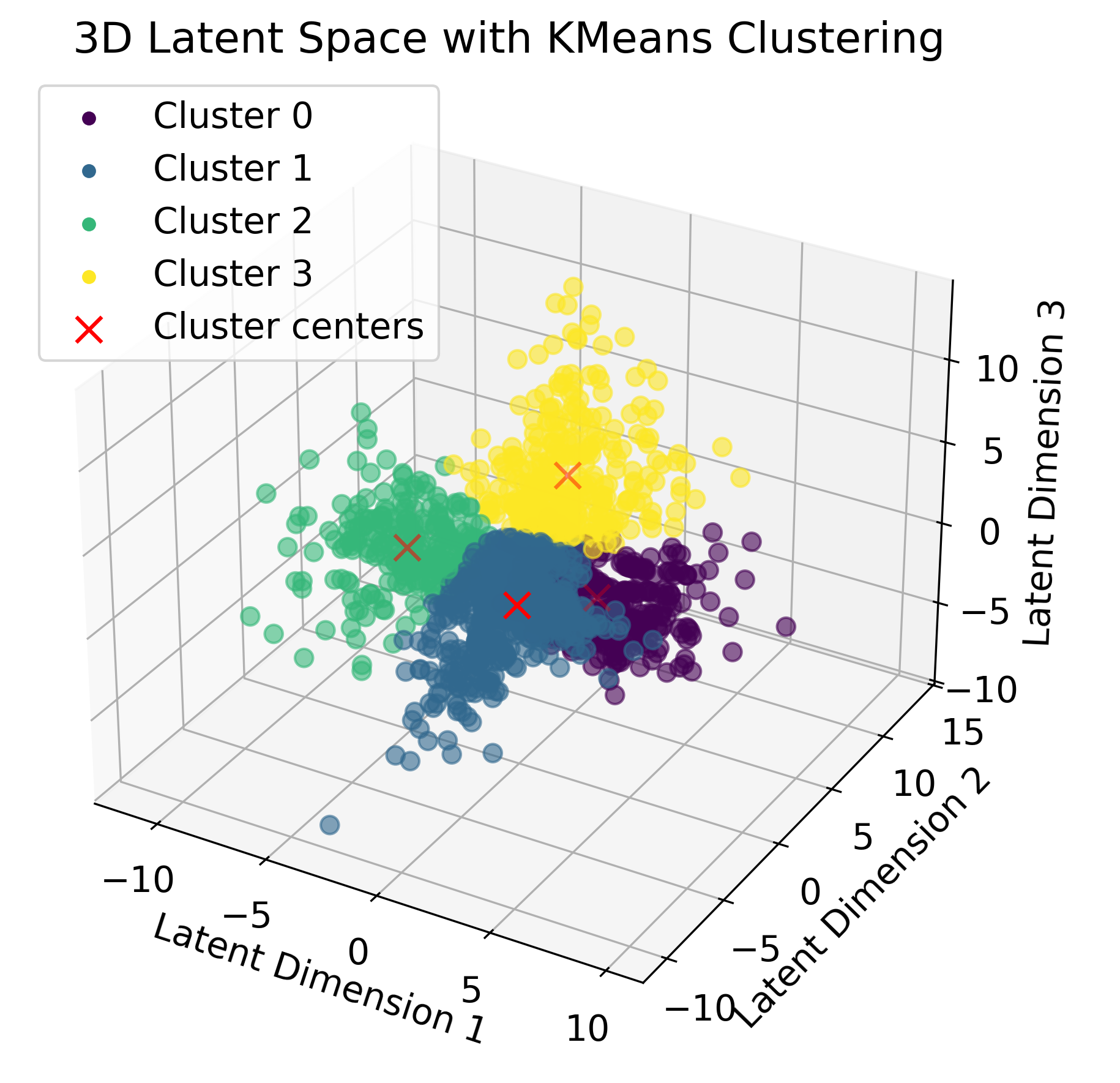Autoencoder-latent space representation of the neural data color-coded by K-means clustering labels.

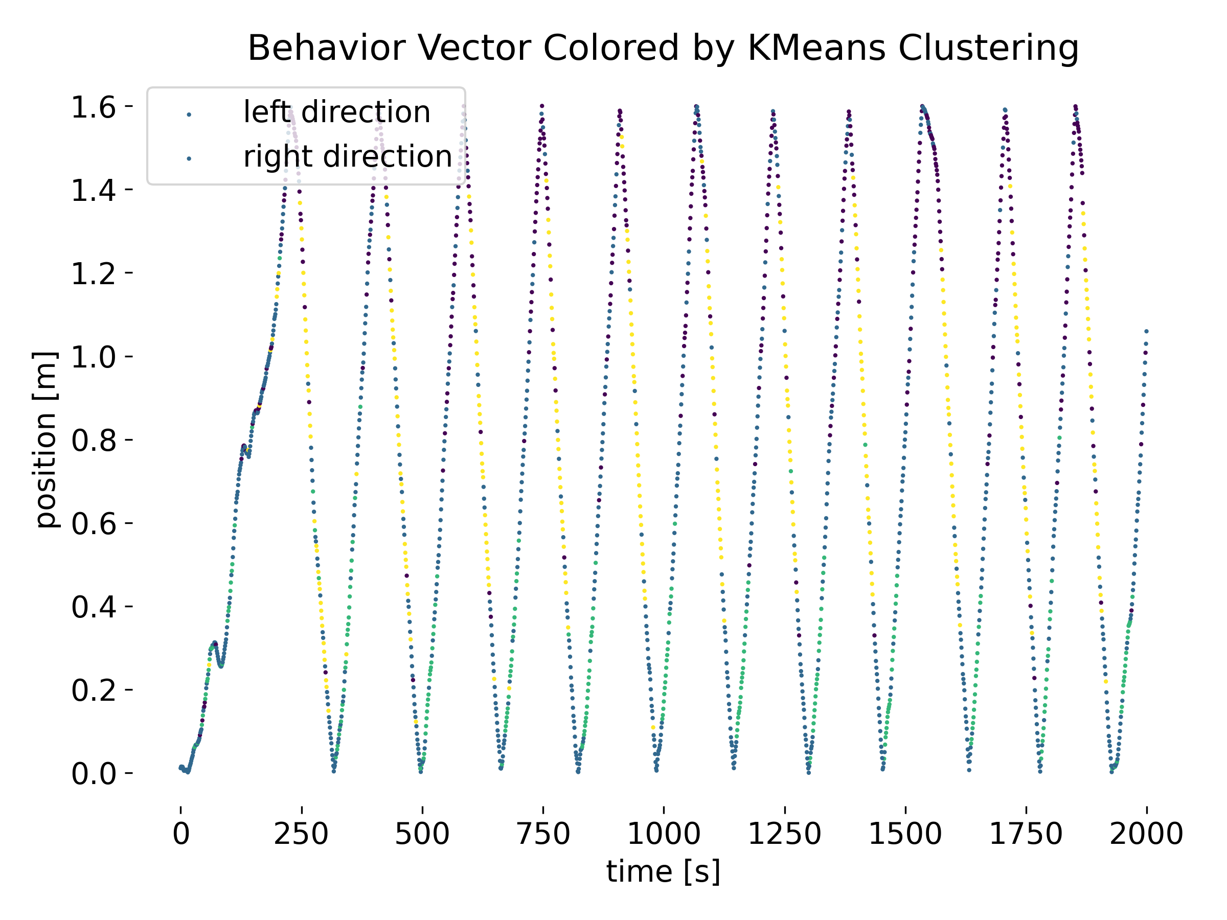‘Phases’ in the behavior vector based on the clusters in the latent space of the autoencoder.

Access the exercise notebook here:

Exercise 1:

Exercise 2: