Excurse: Activation functions and the vanishing gradient problem
This chapter provides a brief overview of activation functions and the so-called vanishing gradient problem. It serves as a supporting chapter for the neural networks that we discuss during the course, providing a theoretical background on these topics and useful background information for understanding the training of deep neural networks.
Activation functions are a crucial component of neural networks, as they introduce non-linearity into the model. The vanishing gradient problem is a common issue in deep neural networks that can hinder the training process. Understanding these concepts is essential for effectively designing and training neural networks.
Activation functions in neural networks
Activation functions play a crucial role in neural networks by introducing non-linearity into the network. Without activation functions, a neural network composed solely of linear transformations (matrix multiplications and additions) would be limited in its ability to model complex data. Specifically, a network with only linear transformations can only represent linear mappings from inputs to outputs, regardless of the number of layers. This makes it incapable of capturing non-linear relationships, which are essential in most real-world applications, such as image recognition, natural language processing, and many others.
Mathematically, consider a neural network where each layer performs a linear transformation on its input:
\[\mathbf{h}^{(l)} = \mathbf{W}^{(l)} \mathbf{h}^{(l-1)} + \mathbf{b}^{(l)}\]where:
- $\mathbf{h}^{(l-1)}$ is the output of the previous layer (or the input data for the first layer),
- $\mathbf{W}^{(l)}$ and $\mathbf{b}^{(l)}$ are the weights and biases for layer $l$.
Without an activation function, the composition of these transformations remains linear. Activation functions, applied element-wise to each neuron’s output, allow the network to learn non-linear decision boundaries and approximate more complex functions:
\[\mathbf{h}^{(l)} = \sigma(\mathbf{W}^{(l)} \mathbf{h}^{(l-1)} + \mathbf{b}^{(l)})\]Here, $\sigma(\cdot)$ is the activation function, which introduces non-linearity into the network. Activation functions are typically applied after the linear transformation in each layer, enabling the network to model complex relationships in the data.
Common Activation Functions
In the following, we will review some commonly used activation functions, including their mathematical properties, advantages, and disadvantages.
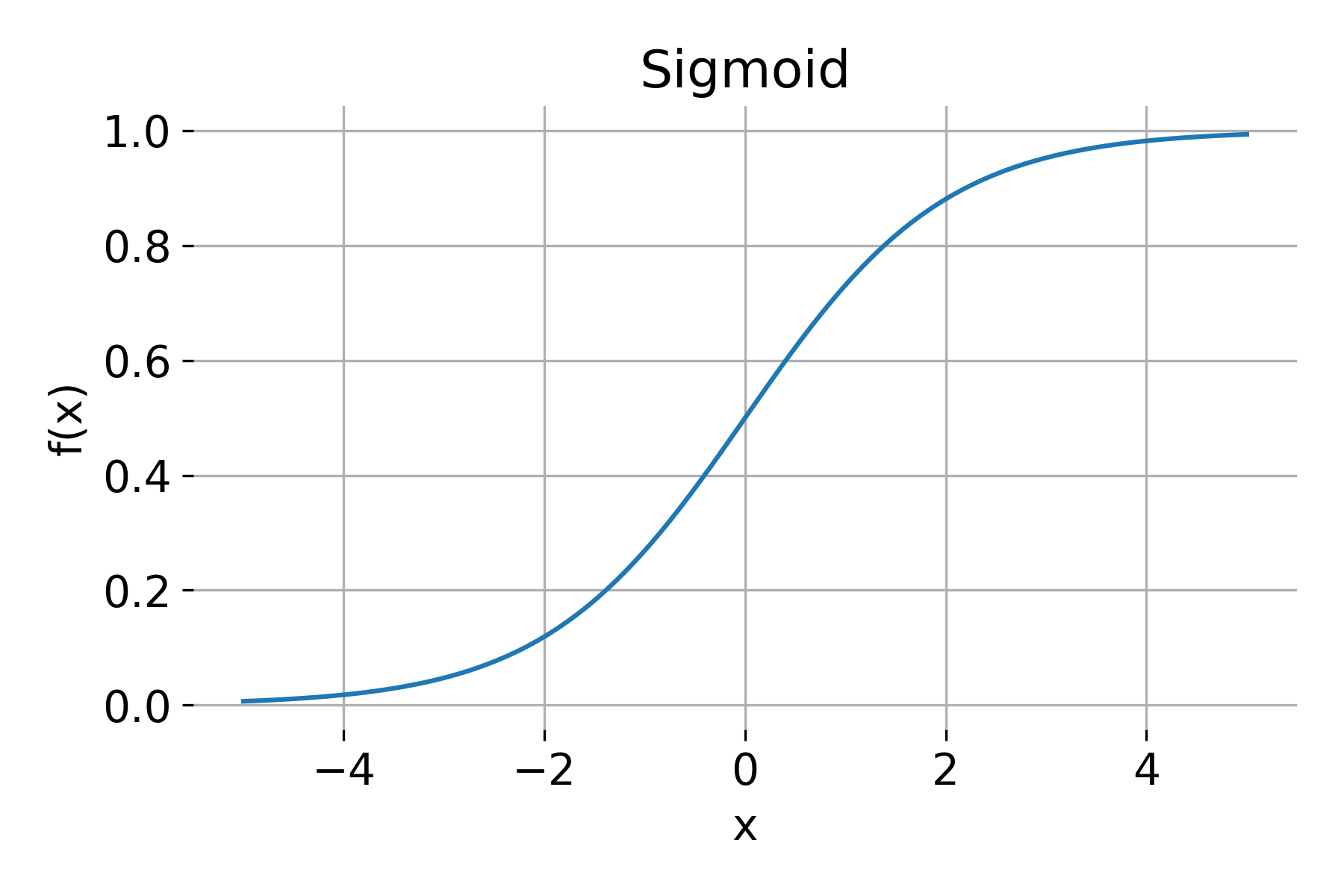
Sigmoid
The sigmoid function is defined as:
\[\sigma(x) = \frac{1}{1 + e^{-x}}\]The sigmoid function has the following properties:
- Range: $(0, 1)$
- Derivative: \(\sigma'(x) = \sigma(x) \cdot (1 - \sigma(x))\)
The sigmoid function squashes the input to a range between 0 and 1, making it suitable for binary classification tasks. However, it has several limitations, such as:
- Vanishing gradients: For large positive or negative values of $x$, the derivative $\sigma’(x)$ approaches zero, which can slow down or even stop the training of deep networks.
- Output range: Its output is not zero-centered, which can cause issues during training, as gradients have consistent signs, leading to slower convergence.
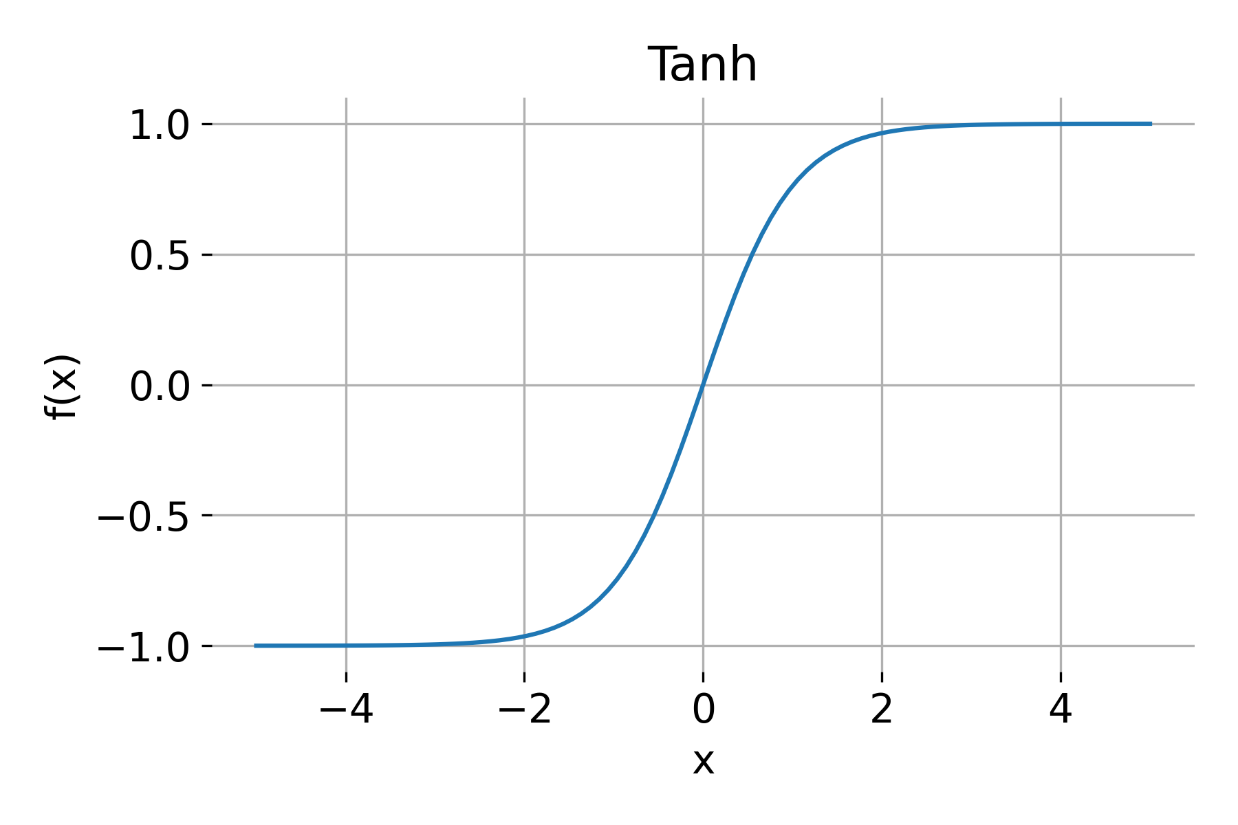
Tanh
The tanh (hyperbolic tangent) function is an improvement over the sigmoid function, defined as:
\[\text{tanh}(x) = \frac{e^x - e^{-x}}{e^x + e^{-x}}\]The properties of the tanh function are:
- Range: $(-1, 1)$
- Derivative: \(\text{tanh}'(x) = 1 - \text{tanh}^2(x)\)
Since tanh outputs values centered around zero, it often leads to faster convergence compared to sigmoid. However, it still suffers from the vanishing gradient problem for large values of $x$.
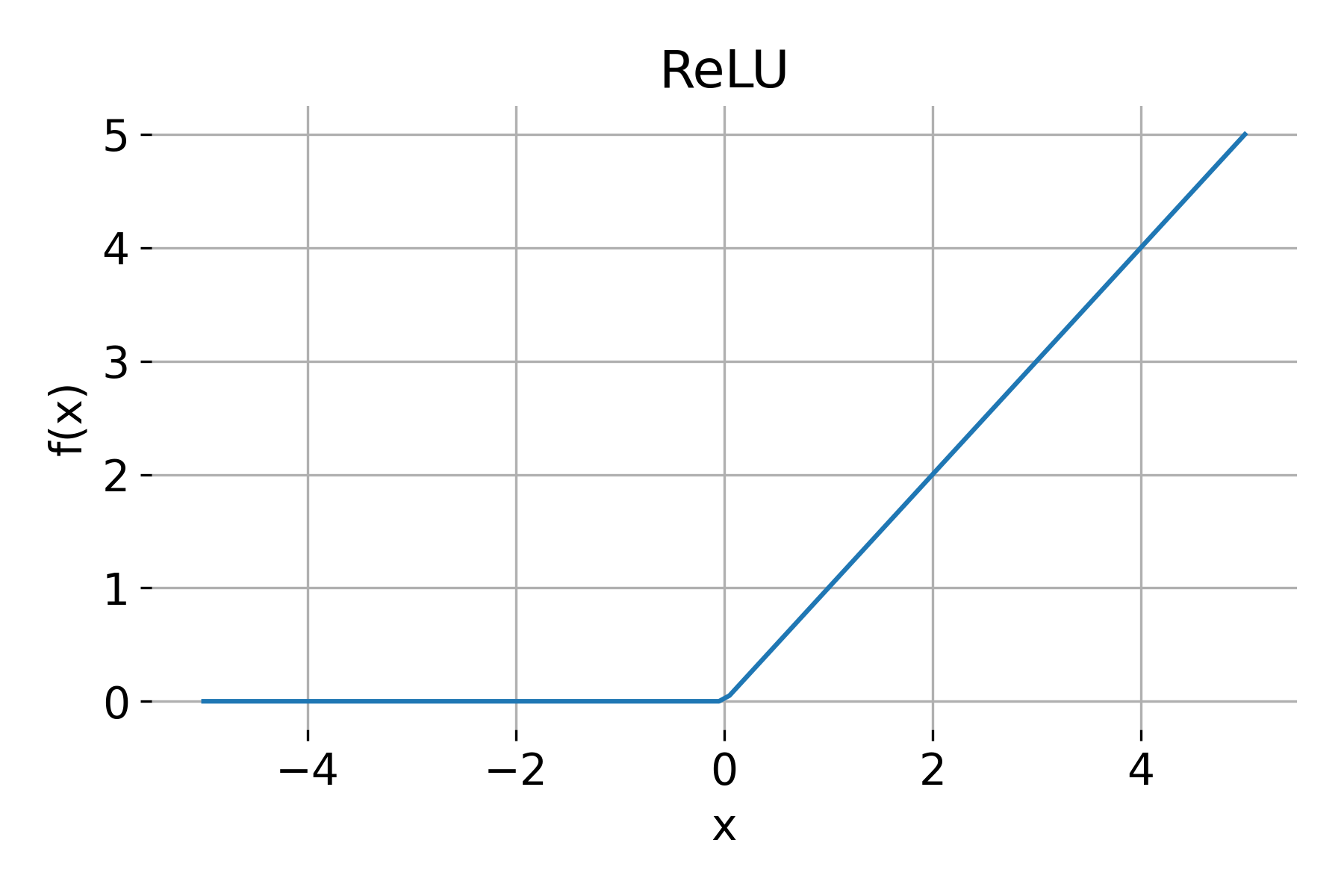
ReLU
The ReLU (Rectified Linear Unit) function is defined as:
\[\text{ReLU}(x) = \max(0, x)\]Properties of ReLU:
- Range: $[0, \infty)$
- Derivative: \(\text{ReLU}'(x) = \begin{cases} 1 & \text{if } x > 0 \\ 0 & \text{if } x \leq 0 \end{cases}\)
ReLU is widely used in hidden layers due to its simplicity and efficiency in training deep networks. Advantages of ReLU include:
- Non-linearity: ReLU introduces non-linearity, allowing the network to learn complex patterns.
- Computational efficiency: ReLU is simple to compute.
- Mitigates vanishing gradient problem: For positive values, gradients do not vanish, enabling faster convergence in deep networks.
However, ReLU has a drawback known as the dying ReLU problem: neurons can “die” if they enter the inactive region (i.e., if $x \leq 0$) and never recover, which can reduce network capacity.
Leaky ReLU
Leaky ReLU addresses the dying ReLU problem by allowing a small, non-zero gradient when $x < 0$: $$
\text{Leaky ReLU}(x) =
\begin{cases}
x & \text{if } x > 0
\alpha x & \text{if } x \leq 0
\end{cases}
$$
where $\alpha$ is a small constant, typically set to 0.01.
Properties:
- Range: $(-\infty, \infty)$
- Derivative: \(\text{Leaky ReLU}'(x) = \begin{cases} 1 & \text{if } x > 0 \\ \alpha & \text{if } x \leq 0 \end{cases}\)
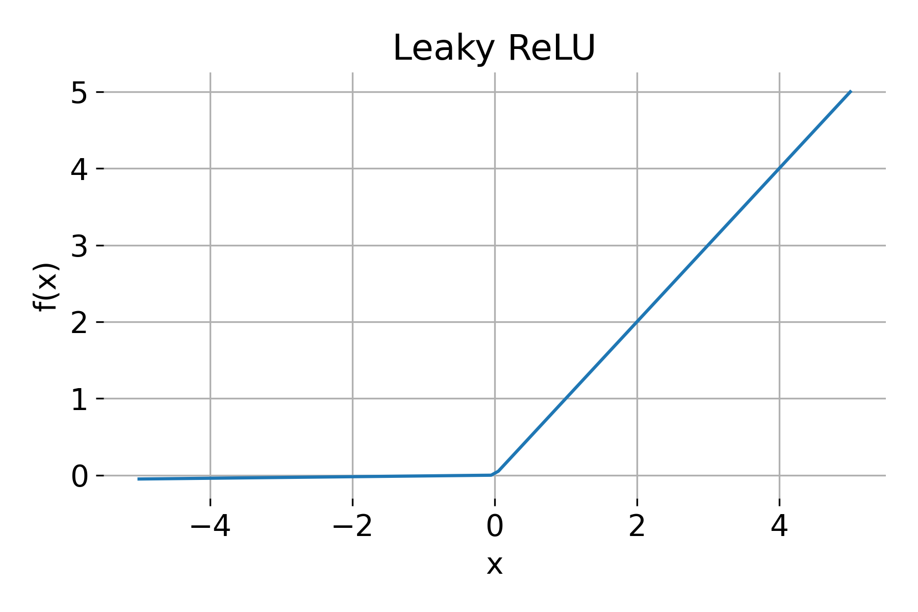
Leaky ReLU activation function.
Leaky ReLU provides a small gradient for negative values, reducing the risk of neurons “dying.”
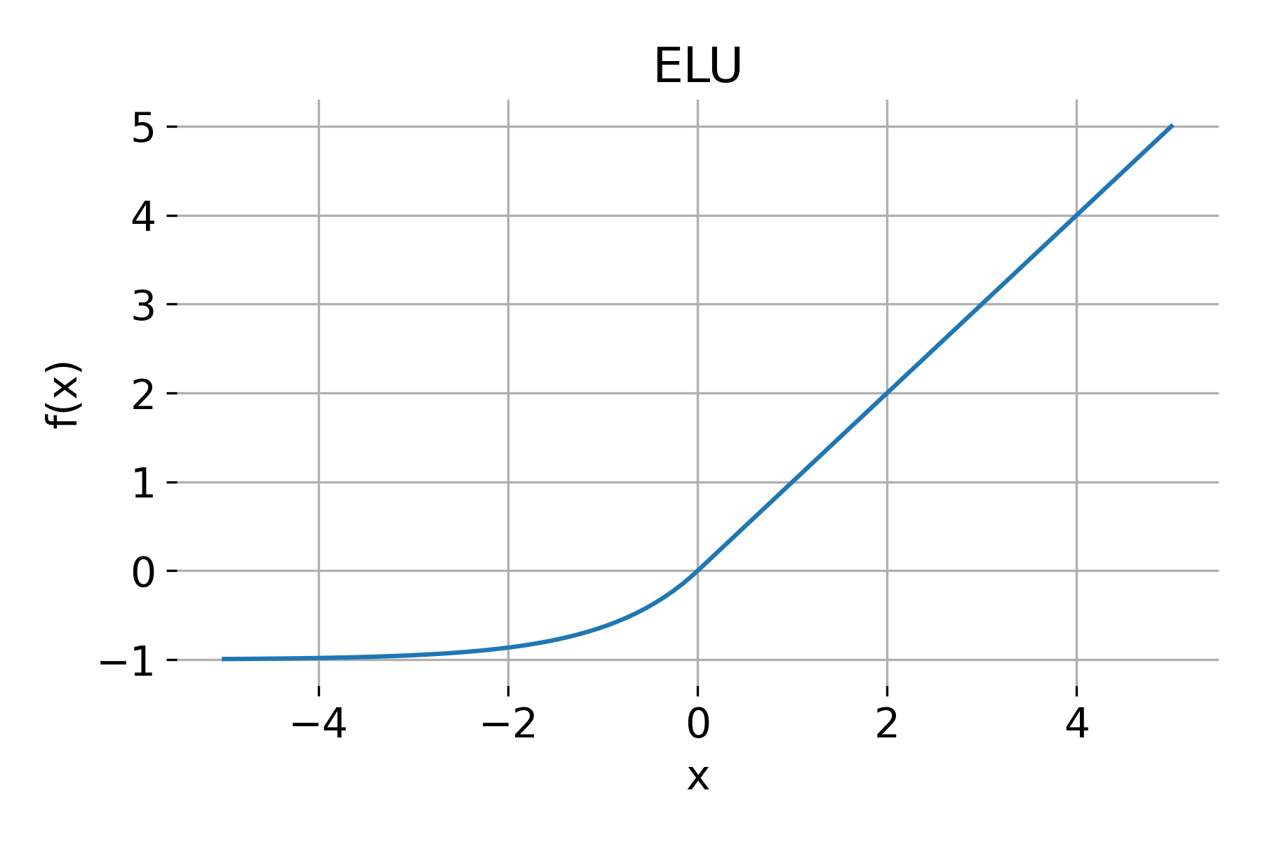
ELU
The ELU (Exponential Linear Unit) function is defined as:
\[\text{ELU}(x) = \begin{cases} x & \text{if } x > 0 \\ \alpha (e^x - 1) & \text{if } x \leq 0 \end{cases}\]Properties:
- Range: $(-\alpha, \infty)$
- Derivative: \(\text{ELU}'(x) = \begin{cases} 1 & \text{if } x > 0 \\ \alpha e^x & \text{if } x \leq 0 \end{cases}\)
ELU has the advantage of producing smoother transitions and retaining small negative values, which can help the network converge faster than ReLU. However, ELU is computationally more expensive.
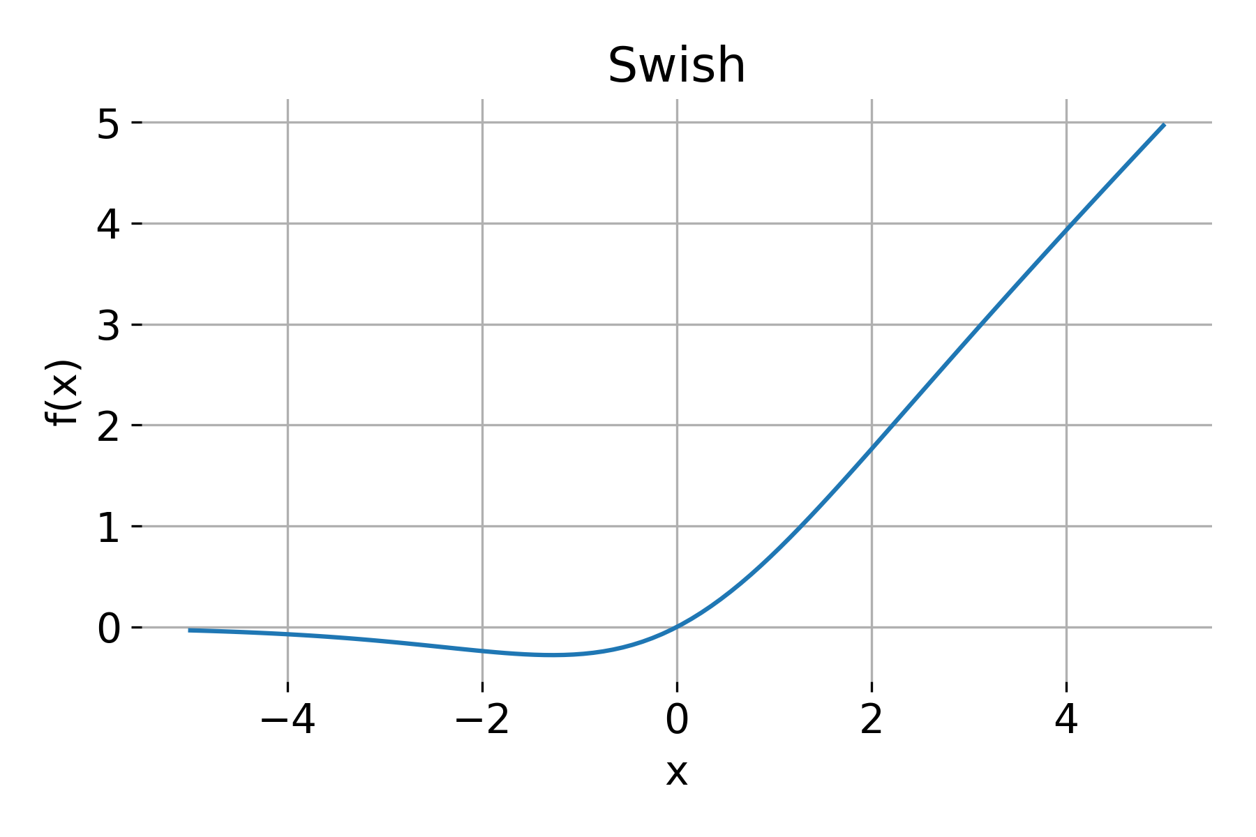
Swish
Swish is a self-gated activation function, defined as:
\[\text{Swish}(x) = x \cdot \sigma(\beta x) = \frac{x}{1 + e^{-\beta x}}\]Properties:
- Range: $(-\infty, \infty)$
- Derivative: Swish’s derivative is more complex but can be computed analytically or using automatic differentiation.
Swish has shown superior performance to ReLU in some deep networks. Its gating mechanism allows smooth gradients, enabling stable training and performance improvements.
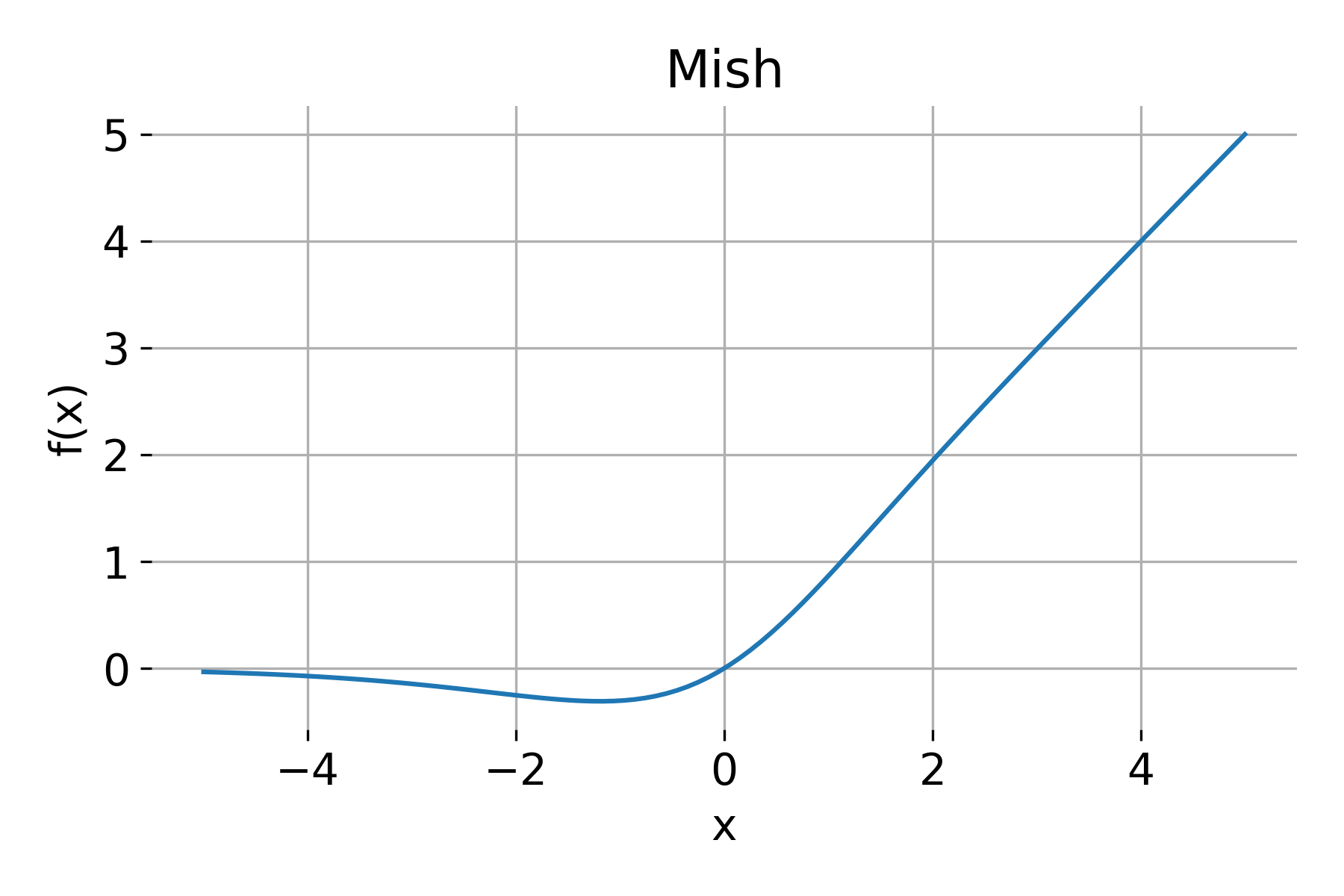
Mish
Mish is defined as:
\[\text{Mish}(x) = x \cdot \text{tanh}(\ln(1 + e^x))\]Properties:
- Range: $(-\infty, \infty)$
- Derivative: Mish’s derivative is complex and often calculated using automatic differentiation frameworks.
Mish is a smooth, non-monotonic function and has been shown to outperform ReLU and Swish in some cases. Its smoothness and non-linearity encourage better gradient flow and can improve generalization.
Softmax
The softmax function is typically used in the output layer for multi-class classification problems. For an input vector $\mathbf{x} = [x_1, x_2, \dots, x_n]$, softmax is defined as:
\[\text{Softmax}(x_i) = \frac{e^{x_i}}{\sum_{j=1}^{n} e^{x_j}}\]Properties:
- Range: $(0, 1)$, with outputs summing to 1
-
Derivative: The derivative is more complex and involves partial derivatives, given by:
\[\frac{\partial \text{Softmax}(x_i)}{\partial x_j} = \text{Softmax}(x_i) \left(\delta_{ij} - \text{Softmax}(x_j)\right)\]where $\delta_{ij}$ is the Kronecker delta, equal to 1 if $i = j$ and 0 otherwise.
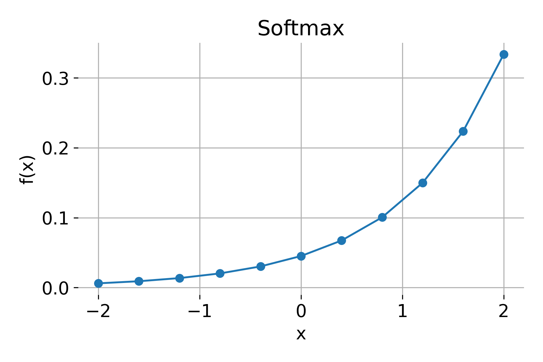
Softmax activation function, evaluated for a vector of logits.
Softmax converts a vector of raw scores (logits) into probabilities that sum to 1, making it suitable for classification tasks.
Summary of activation functions
| Activation | Range | Derivative | Advantages | Disadvantages |
|---|---|---|---|---|
| Sigmoid | $(0, 1)$ | $\sigma(x)(1 - \sigma(x))$ | Smooth, probabilistic output | Vanishing gradients, not zero-centered |
| Tanh | $(-1, 1)$ | $1 - \text{tanh}^2(x)$ | Zero-centered, smooth | Vanishing gradients |
| ReLU | $[0, \infty)$ | \(\begin{cases} 1 & x > 0 \\ 0 & x \leq 0 \end{cases}\) | Simple, effective, mitigates vanishing gradient | Dying ReLU problem |
| Leaky ReLU | $(-\infty, \infty)$ | \(\begin{cases} 1 & x > 0 \\ \alpha & x \leq 0 \end{cases}\) | Solves dying ReLU | Requires tuning $\alpha$ |
| ELU | $(-\alpha, \infty)$ | Smooth, adaptable | Fast convergence, smooth | Computationally expensive |
| Swish | $(-\infty, \infty)$ | Complex | Smooth gradients, self-gated | Computationally more complex |
| Mish | $(-\infty, \infty)$ | Complex | Smooth, non-monotonic | Computationally more complex |
| Softmax | $(0, 1)$, sums to 1 | Complex | Converts to probability | Limited to output layer |
Each activation function has its advantages and disadvantages, and the choice of activation depends on the specific neural network architecture and task. Experimentation and empirical tuning often guide the selection of an appropriate activation function for deep learning models.
The vanishing gradient problem
The vanishing gradient problem is a phenomenon that arises during the training of deep neural networks. When this problem occurs, the gradients of the loss function with respect to the parameters (weights) become exceedingly small as they are propagated back through the layers of the network. As a result, the network parameters in earlier layers are updated very slowly, leading to slow convergence, poor performance, or even complete failure to learn in deep networks.
Why do gradients vanish?
To understand why gradients vanish, let’s review how training works. Neural networks use backpropagation to compute the gradients of the loss function with respect to each parameter. The chain rule of calculus is applied layer by layer from the output layer back to the input layer. For a network with $L$ layers, this process involves a chain of partial derivatives:
\[\frac{\partial L}{\partial \mathbf{W}^{(i)}} = \frac{\partial L}{\partial \mathbf{h}^{(L)}} \cdot \frac{\partial \mathbf{h}^{(L)}}{\partial \mathbf{h}^{(L-1)}} \cdot \dots \cdot \frac{\partial \mathbf{h}^{(i+1)}}{\partial \mathbf{h}^{(i)}} \cdot \frac{\partial \mathbf{h}^{(i)}}{\partial \mathbf{W}^{(i)}}\]Here, $\frac{\partial \mathbf{h}^{(i+1)}}{\partial \mathbf{h}^{(i)}}$ is the derivative of the activation of layer $i+1$ with respect to the activation of layer $i$. When deep networks are trained, the gradients are multiplied many times through layers in the network. If the derivatives are small (less than 1), the product of these derivatives decreases exponentially as the depth of the network increases, driving the gradient toward zero in earlier layers.
Role of activation functions
The choice of activation function plays a crucial role in the vanishing gradient problem. Activation functions with small gradients, like sigmoid and tanh, are particularly susceptible to this issue:
For sigmoid:
\[\sigma'(x) = \sigma(x) (1 - \sigma(x))\]When $x$ is large (positive or negative), $\sigma(x)$ saturates near 0 or 1, and $\sigma’(x)$ becomes very close to 0. This can lead to vanishing gradients in deeper layers.
For tanh:
\[\text{tanh}'(x) = 1 - \text{tanh}^2(x)\]Similarly, $\text{tanh}’(x)$ becomes very small for large values of $x$, causing gradients to vanish.
This is why ReLU (Rectified Linear Unit) has become popular for hidden layers in deep networks. ReLU has a gradient of 1 for positive inputs, which helps maintain gradients during backpropagation and reduces the likelihood of vanishing gradients. However, ReLU introduces the dying ReLU problem, where neurons can become inactive if their inputs are negative, which causes their gradients to be zero.
Consequences
The vanishing gradient problem can have several consequences for deep neural networks:
- Slow Training: With small gradients, the weights in earlier layers are updated very slowly, making it difficult for the network to converge within a reasonable timeframe.
- Poor Performance: If the network can’t learn effectively, it may fail to find a good representation of the data, leading to poor generalization and low accuracy.
- Unlearned Early Layers: Layers closer to the input may learn very slowly or not at all, effectively limiting the network’s capacity to learn complex hierarchical features.
Solutions
Several techniques have been developed to mitigate the vanishing gradient problem:
Use of activation functions like ReLU and variants
As mentioned, ReLU helps reduce the vanishing gradient problem by providing a constant gradient for positive values. Variants like Leaky ReLU, ELU, and Mish further enhance gradient flow by allowing small gradients for negative inputs.
Weight initialization techniques
Proper weight initialization can help maintain the gradient’s scale as it propagates through layers.
Xavier (Glorot) Initialization: Initializes weights to keep the variance of activations similar across layers. Typically used with sigmoid or tanh activations.
\[W \sim \mathcal{U} \left(-\frac{\sqrt{6}}{\sqrt{n_{\text{in}} + n_{\text{out}}}}, \frac{\sqrt{6}}{\sqrt{n_{\text{in}} + n_{\text{out}}}}\right)\]He Initialization: Specifically designed for ReLU networks, He initialization sets weights with larger variance, helping to sustain gradients across layers.
\[W \sim \mathcal{N} \left(0, \frac{2}{n_{\text{in}}}\right)\]Batch normalization
Batch Normalization normalizes the activations of each layer by adjusting and scaling them. This helps control the internal covariate shift (changes in the distribution of layer inputs over training) and can stabilize gradients.
Batch normalization also reduces the dependency on the initial weights and helps the network learn more quickly and effectively.
Residual connections
Residual Networks (ResNets) introduce skip connections where the input to a layer is added directly to its output. This enables gradients to flow directly through the network, bypassing certain layers, which helps alleviate the vanishing gradient problem.
Mathematically, a residual block is:
\[\mathbf{h}^{(l+1)} = \mathbf{h}^{(l)} + f(\mathbf{h}^{(l)}, \mathbf{W}^{(l)})\]This formulation allows gradients to flow backward through the shortcut path, ensuring they do not vanish as easily in deeper layers.
Gradient Clipping
In some cases, gradient clipping is applied to limit the size of gradients, especially in recurrent neural networks, to prevent them from becoming too large (which addresses the related exploding gradient problem).
