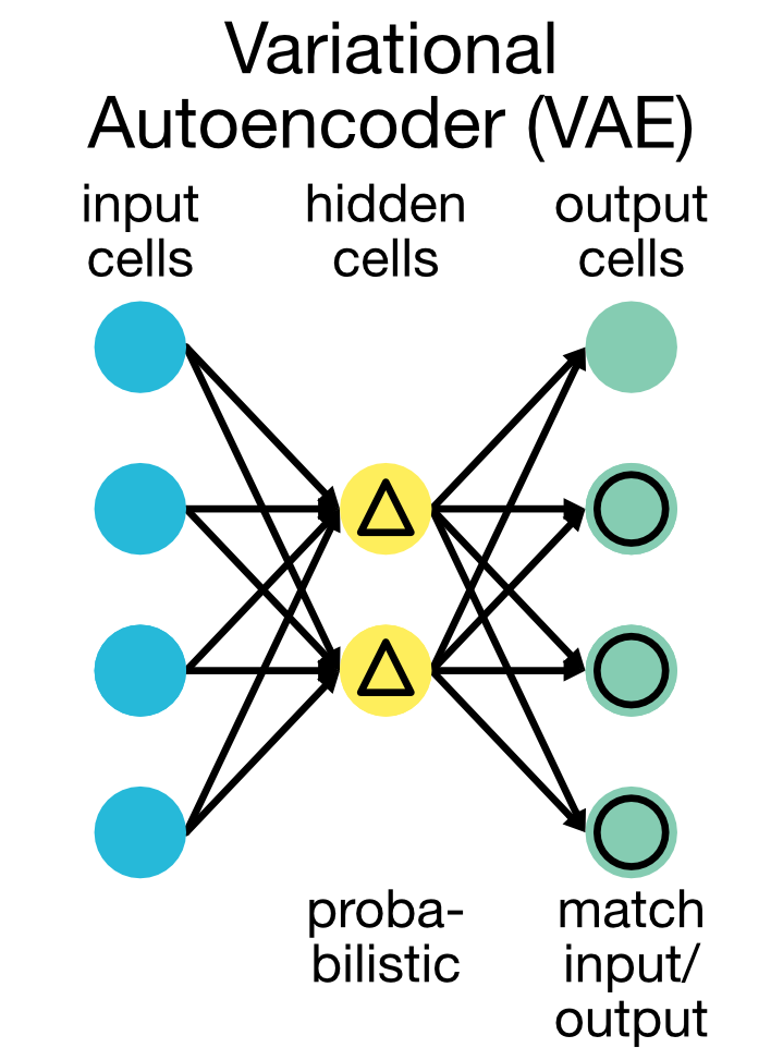
Variational Autoencoders (VAE)

Variational Autoencoders (VAEs) are a class of probabilistic generative models. Unlike traditional autoencoders that produce a deterministic latent space, VAEs introduce a probabilistic framework, enabling meaningful sampling and generation of new data. This necessitates a shift in perspective — from fixed latent vectors to distributions over latent spaces. To motivate this shift and its advantages, we’ll start by revisiting traditional autoencoders, introduce Bayes’ theorem in the context of deep learning, and discuss the critical differences between traditional autoencoders and VAEs.

Motivation

In traditional autoencoders, we map data $x$ to a lower-dimensional latent space representation $z$ through an encoder network. The decoder then uses this deterministic $z$ to reconstruct the original input $x$, minimizing reconstruction error. However, this deterministic approach has limitations:

• limited generative capability: Since the encoder learns fixed mappings for each input, we cannot generate meaningful new samples by sampling from the latent space.
• non-continuous latent space: The latent representations may be distributed in an arbitrary fashion across the latent space, making interpolation between points meaningless.

To address these issues, we can reframe the latent space probabilistically. Instead of mapping each input $x$ to a single point in latent space, we can map it to a distribution over possible latent representations. This shift introduces flexibility and opens up the model to probabilistic reasoning — specifically, by employing Bayes’ theorem, we can connect observed data to latent variables.

Bayes’ theorem

The goal of a VAE is to learn the underlying data distribution $P(x)$ by introducing a latent variable $z$ that captures essential characteristics of $x$. To achieve this, we need to compute the posterior distribution $P(z|x)$, representing the probability of a latent representation $z$ given observed data $x$. Bayes’ theorem gives us:

\[P(z|x) = \frac{P(x|z) \cdot P(z)}{P(x)}\]

where:

• $P(z|x)$: The posterior distribution of the latent variables given data $x$.
• $P(x|z)$: The likelihood—the probability of observing $x$ given $z$.
• $P(z)$: The prior distribution over latent variables, usually set to a standard Gaussian $\mathcal{N}(0, I)$ to enforce a structured, continuous latent space.
• $P(x)$: The evidence or marginal likelihood, which normalizes the distribution.

Bayes’ theorem example: Cough and cold

To make Bayes’ theorem more relatable, let’s use a simple everyday example involving the probability of having a cold given a symptom.

Imagine it’s flu season, and you wake up with a cough. You’re wondering if this cough means you likely have a cold. Let’s break this down using Bayes’ theorem.

Let’s set up the events:

• Event A: You have a cold.
• Event B: You have a cough.

We want to find the probability of having a cold given that you have a cough, written as $P(A|B)$.

To use Bayes’ theorem, we need:

• $P(A)$: The probability of having a cold on any given day (maybe based on flu season statistics).
• $P(B|A)$: The probability of having a cough if you have a cold.
• $P(B)$: The overall probability of having a cough (whether you have a cold or not).

Let’s assign some hypothetical values:

• $P(A) = 0.1$: There’s a 10% chance of having a cold on any given day.
• $P(B|A) = 0.8$: If you have a cold, there’s an 80% chance you’ll have a cough.
• $P(B) = 0.3$: On any given day, there’s a 30% chance of having a cough (since other things like allergies can also cause coughing).

Bayes’ theorem now states:

\[P(A|B) = \frac{P(B|A) \cdot P(A)}{P(B)}\]

Substitute the values:

\[P(\text{Cold | Cough}) = \frac{0.8 \cdot 0.1}{0.3} = \frac{0.08}{0.3} \approx 0.27\]

So, given that you have a cough, there’s a 27% chance that you have a cold. This probability might seem low, but it reflects the fact that coughing can happen for reasons other than a cold, and not every cough should immediately raise high concerns.

This example is simple but effective because it emphasizes conditional probability: the probability of having a cold changes when you know you have a cough.

Since calculating $P(x)$ is computationally intractable (as it requires summing over all possible latent variables), we instead approximate $P(z|x)$ with a simpler variational distribution $q(z|x)$. This approximation forms the foundation of the variational autoencoder, where the encoder learns $q(z|x)$, and the decoder approximates $P(x|z)$.

Mathematical formulation

The VAE architecture consists of an encoder, a latent space with a probabilistic distribution, and a decoder. In the following, we break down the these key components:

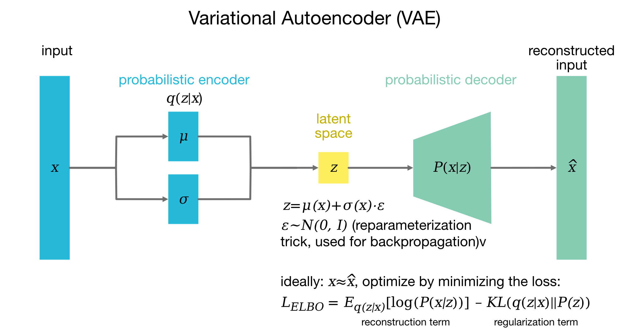Variational Autoencoder (VAE) architecture. In a VAE, the input data $x$ is first processed by a probabilistic encoder, which maps it to a latent representation $z$ through the parameters $\mu(x)$ (mean) and $\sigma(x)$ (standard deviation). These parameters define a Gaussian distribution $q(z|x) = \mathcal{N}(\mu(x), \sigma(x)^2)$ from which $z$ is sampled. To allow gradients to flow through the stochastic sampling, the reparameterization trick is used (see below), representing $z$ as $z = \mu(x) + \sigma(x) \cdot \epsilon$, where $\epsilon \sim \mathcal{N}(0, I)$ introduces controlled randomness. This transformation enables backpropagation through the encoder parameters $\mu(x)$ and $\sigma(x)$. The decoder then reconstructs the original input $x$ by generating a distribution $P(x|z)$ over possible outputs given $z$. The reconstruction $\hat{x}$ represents the model’s best approximation of the input $x$. The VAE is trained by optimizing the Evidence Lower Bound (ELBO) loss, which consists of two parts: (1) the reconstruction term, $\mathbb{E}_{q(z|x)}[\log P(x|z)]$, which encourages the output $\hat{x}$ to be similar to the input $x$; and (2) the KL divergence term, $\text{KL}(q(z|x) || P(z))$, which regularizes $z$ to follow a standard Gaussian prior $P(z) = \mathcal{N}(0, I)$, encouraging a more structured and disentangled latent space. By minimizing the ELBO, the VAE learns both to encode data into a meaningful latent space and to generate realistic reconstructions. Figure adapted from Lilian Wang’s blogꜛ.

Encoder network: $q(z|x)$

The encoder maps input $x$ to the parameters of a latent Gaussian distribution:

\[q(z|x) = \mathcal{N}(z; \mu(x), \sigma^2(x))\]

where:

• Weights and biases of the encoder layers are denoted by $W$ and $b$, which are learned during training.
• Feature extraction layers: The encoder typically uses fully connected or convolutional layers to process input data, with a nonlinear activation function such as ReLU.
• Latent parameters: The encoder outputs two vectors, $\mu(x)$ (mean) and $\log \sigma^2(x)$ (log-variance), which are mapped through a fully connected layer followed by activation functions.

For each data point $x$, the encoder produces:

\[\begin{align*} \mu(x) &= W_\mu \cdot \phi(x) + b_\mu \\ \log \sigma^2(x) &= W_{\sigma} \cdot \phi(x) + b_{\sigma} \end{align*}\]

where $\phi(x)$ represents the features extracted by earlier layers of the encoder.

Latent space and reparameterization trick

To sample $z$ in a differentiable way, we use the reparameterization trick. Instead of sampling $z$ directly from $\mathcal{N}(\mu, \sigma^2)$, we rewrite $z$ as:

\[z = \mu(x) + \sigma(x) \cdot \epsilon\]

where $\epsilon \sim \mathcal{N}(0, I)$, with $I$ being the identity matrix (thus, $\epsilon$ is drawn from a multivariate normal distribution with mean $0$ and covariance $I$, the identity matrix). This formulation makes $z$ a deterministic function of $\mu(x)$, $\sigma(x)$, and $\epsilon$, enabling backpropagation.

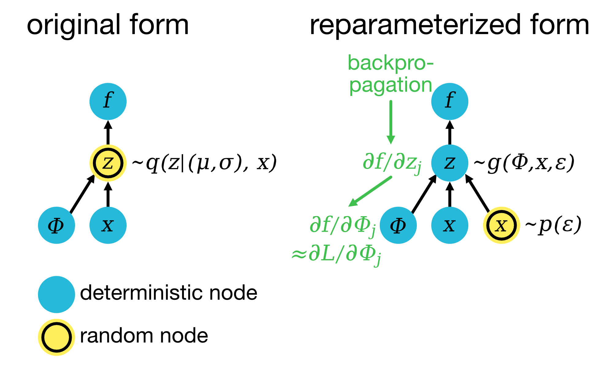Reparameterization trick: In the original form (left), the latent variable $z$ is sampled from an approximate posterior distribution $q(z|\mu, \sigma)$, where $\mu$ and $\sigma$ are parameters computed based on the input data $x$, determined by the encoder parameters $\Phi=\Phi(\mu, \sigma)$. The function $f$ represents the decoder, which reconstructs the output. Due to the stochastic sampling of $z$, it is challenging to backpropagate gradients through this path, which would prevent learning the parameters $\Phi$ via gradient descent. In the reparameterized form (right), we transform the sampling operation into a deterministic one by introducing a random variable $\epsilon$ (typically sampled from a standard normal distribution, $p(\epsilon) \sim \mathcal{N}(0, 1)$). Here, $z$ is expressed as a function of $\epsilon$, the input $x$, and encoder parameters $\Phi(\mu, \sigma)$: $z = g(\Phi, x, \epsilon) = \mu + \sigma \cdot \epsilon$. This transformation allows gradients to flow through $z$ by reparameterizing it as a differentiable function of $\Phi$, making it possible to optimize the VAE’s objective function, the Evidence Lower Bound (ELBO, denoted as $L$ in the figure), by computing $\frac{\partial L}{\partial \Phi}$ via backpropagation through $g(\Phi, x, \epsilon)$. Figure adapted from Lilian Wang’s blogꜛ and Kingma & Welling (2014)ꜛ.

Decoder network: $P(x|z)$

The decoder reconstructs $x$ from $z$ by approximating $P(x|z)$. It typically uses:

• Fully connected layers that mirror the encoder structure.
• An output layer with a sigmoid activation for bounded output, or no activation for unbounded data.

The decoder network takes a sampled $z$ and reconstructs $x$ as:

\[\hat{x} = f(W_{\text{dec}} \cdot z + b_{\text{dec}})\]

Loss function: Evidence Lower Bound (ELBO)

To train a VAE, we maximize the Evidence Lower Bound (ELBO), an approximation to the log-likelihood of the data:

\[\mathcal{L}_{\text{ELBO}} = \mathbb{E}_{q(z|x)} \left[ \log P(x|z) \right] - \text{KL}(q(z|x) || P(z))\]

This formulation consists of two terms:

1. Reconstruction Loss $\mathbb{E}_{q(z|x)} \left[ \log P(x|z) \right]$: Measures how accurately the decoder reconstructs $x$ from $z$.
2. Kullback-Leibner (KL) Divergence $\text{KL}(q(z|x) || P(z))$: Regularizes the latent space by ensuring $q(z|x)$ is close to the prior $P(z)$.

The KL divergence term encourages the latent space to be structured and continuous, facilitating meaningful sampling and interpolation. It is defined as:

\[\text{KL}(q(z|x) || P(z)) = -\frac{1}{2} \sum_{j=1}^{J} \left(1 + \log((\sigma_j)^2) - (\mu_j)^2 - (\sigma_j)^2 \right)\]

where $J$ is the dimensionality of the latent space, and $\mu_j$ and $\sigma_j$ are the mean and standard deviation of the $j$-th dimension of $q(z|x)$ (the encoder output).

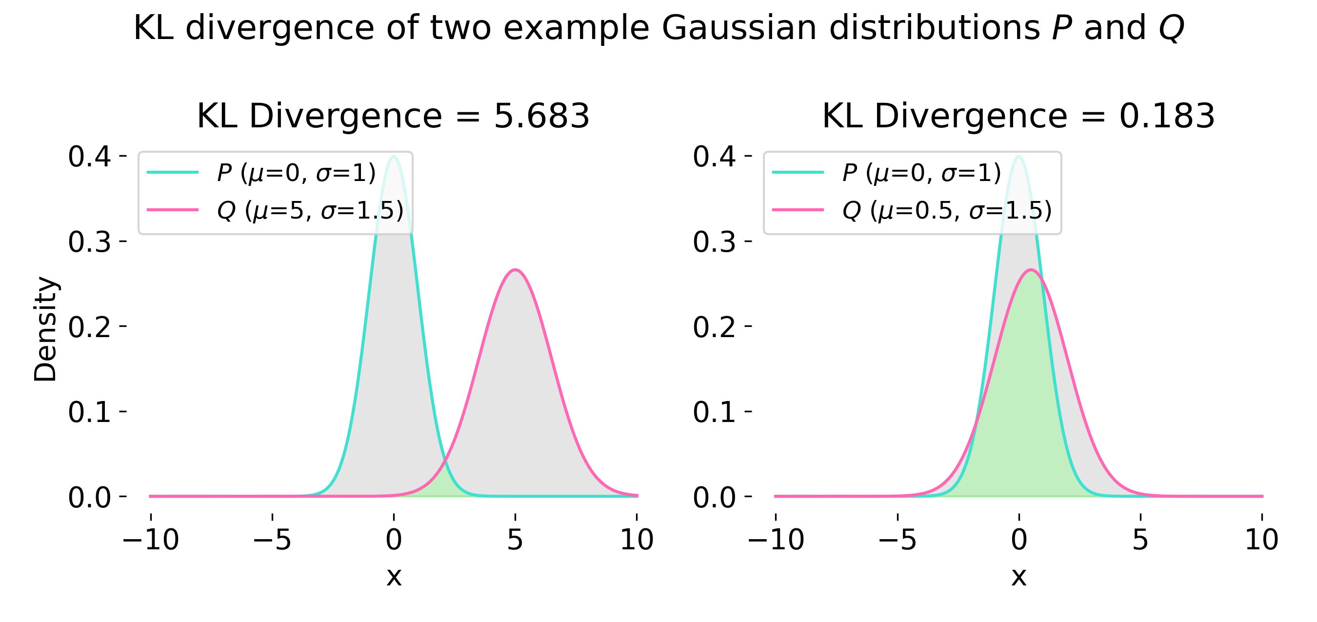
Example of Kullback-Leibner (KL) divergence calculation for two 1D Gaussian distributions $P$ and $Q$ (with $P \neq Q$). The KL divergence measures the difference between the two distributions, which is larger when they are more dissimilar (left), and smaller when they are similar (right). In case of VAE, the goal is to minimize this difference.

The total VAE loss combines both terms (Reconstruction Loss + KL Divergence):

\[\mathcal{L}_{\text{VAE}} = -\mathcal{L}_{\text{ELBO}} = -\mathbb{E}_{q(z|x)} \left[ \log P(x|z) \right] + \text{KL}(q(z|x) || P(z))\]

VAE network architecture

The encoder of a VAE typically consists of fully connected or convolutional layers, followed by two fully connected layers that output the mean $\mu(x)$ and log-variance $\log \sigma^2(x)$ of the latent distribution.

Example:

• Input layer: Takes input $x$.
• Feature extraction layers: Multiple fully connected or convolutional layers with ReLU activations.
• Latent parameters: Two fully connected layers producing $\mu(x)$ and $\log \sigma^2(x)$, representing the mean and variance of $q(z|x)$.

The decoder network mirrors the encoder structure, with fully connected layers that reconstruct the input $x$ from the sampled $z$.

Example:

• Latent input layer: Takes sampled $z$.
• Upsampling layers: Fully connected layers that mirror the encoder structure.
• Output layer: Produces $\hat{x}$, with a sigmoid activation for normalized data or no activation for unbounded data.

General PyTorch implementation

Below is a general implementation of a VAE using PyTorch.

We start with the VAE class definition. This class will consist of the encoder, decoder, and the forward method that combines them. The encoder consists of two fully connected layers that output the mean and log-variance of the latent distribution. The decoder mirrors the encoder structure, reconstructing the input from the sampled latent variable. The forward method combines the encoder and decoder, sampling $z$ from the encoder output, and reconstructing $x$ using the decoder. Note, that we use the reparameterization trick to sample $z$.

import torch
import torch.nn as nn
import torch.optim as optim

class VAE(nn.Module):
    def __init__(self, input_dim, latent_dim):
        super(VAE, self).__init__()
        # encoder layers:
        self.fc1 = nn.Linear(input_dim, 128)
        self.relu1 = nn.ReLU()
        self.fc2_mu = nn.Linear(128, latent_dim)
        self.fc2_logvar = nn.Linear(128, latent_dim)
        
        # decoder layers:
        self.fc3 = nn.Linear(latent_dim, 128)
        self.relu2 = nn.ReLU()
        self.fc4 = nn.Linear(128, input_dim)
        self.sigmoid = nn.Sigmoid()

    def encode(self, x):
        h1 = self.relu1(self.fc1(x))
        return self.fc2_mu(h1), self.fc2_logvar(h1)

    def reparameterize(self, mu, logvar):
        std = torch.exp(0.5 * logvar)
        eps = torch.randn_like(std)
        return mu + eps * std

    def decode(self, z):
        h3 = self.relu2(self.fc3(z))
        return self.sigmoid(self.fc4(h3))

    def forward(self, x):
        mu, logvar = self.encode(x)
        z = self.reparameterize(mu, logvar)
        return self.decode(z), mu, logvar

Next, we need to define the loss function. The VAE loss consists of two terms: the reconstruction loss and the KL divergence. As reconstruction loss, we use the binary cross-entropy loss (BCE, $\log P(x|z)$) since the input data is binary. The BCE loss measures the difference between the reconstructed input and the original input, while the KL divergence regularizes the latent space. The total loss is the sum of these two terms:

# loss function:
def vae_loss(recon_x, x, mu, logvar):
    bce_loss = nn.BCELoss(reduction='sum')
    BCE = bce_loss(recon_x, x)
    KLD = -0.5 * torch.sum(1 + logvar - mu.pow(2) - logvar.exp())
    return BCE + KLD

BCE alternatives for different data types: If the data is continuous, then modeling $P(x∣z)$ with a Gaussian distribution is more appropriate. In that case, the reconstruction loss is often represented as a Mean Squared Error (MSE) loss between $x$ and the reconstructed $\hat{x}$: $\mathbb{E}_{q(z∣x)}[\log P(x∣z)] \approx -\text{MSE}(x, \hat{x})$. In practice, if we’re working with binary or normalized (e.g., pixel values between 0 and 1) image data, BCE is commonly used as the reconstruction loss. For other types of data, or if the data distribution is approximately Gaussian, MSE may be used instead.

Once you have defined the VAE class and the loss function, you can instantiate the model and optimizer and train the VAE using the following code snippets:

# model and optimizer:
input_dim = 784  # example e.g. for MNIST flattened input
latent_dim = 20
model = VAE(input_dim, latent_dim)
optimizer = optim.Adam(model.parameters(), lr=1e-3)

# training loop:
epochs = 10  # example epoch count
for epoch in range(epochs):
    model.train()
    train_loss = 0
    for batch_idx, (data, _) in enumerate(train_loader):
        data = data.view(-1, input_dim)
        optimizer.zero_grad()
        recon_batch, mu, logvar = model(data)
        loss = vae_loss(recon_batch, data, mu, logvar)
        loss.backward()
        train_loss += loss.item()
        optimizer.step()
        
    print(f"Epoch {epoch + 1}/epochs, Loss: {train_loss / len(train_loader.dataset):.4f}")

Advantages and disadvantages

Advantages:

• Structured latent space: The KL divergence regularizes the latent space, encouraging continuity and facilitating meaningful sampling and interpolation.
• Generative capability: VAEs can generate realistic new samples by sampling from the latent space.

Disadvantages:

• Less sharp reconstructions: Compared to GANs (Generative Adversarial Networks), VAEs often produce blurrier reconstructions due to the KL regularization.
• Training instability: Balancing the reconstruction and KL terms can be challenging, requiring careful tuning.

VAE variants

There are several variants of VAEs tailored for specific applications or to enhance specific properties. A common variant is the ** $\beta$-VAE**, which introduces a parameter $\beta$ to control the weight of the KL divergence term:

\[\mathcal{L}_{\text{VAE}} = -\mathbb{E}_{q(z|x)} \left[ \log P(x|z) \right] + \beta \, \text{KL}(q(z|x) || P(z))\]

Larger $\beta$ encourages disentangled representations in the latent space but may sacrifice reconstruction quality.

Other variants include

• Conditional VAEs (CVAE),
• Hierarchical VAEs (HVAE), and
• Vector Quantized VAEs (VQ-VAE),

each tailored for specific applications.

Summary

VAEs are a probabilistic extension of traditional autoencoders that use Bayes’ theorem and the variational approximation to model data distributions in a structured latent space. By regularizing the latent space with a KL divergence, VAEs enable generative modeling, representation learning, and structured interpolation. With variants like $\beta$-VAEs, the model’s flexibility expands, making it a powerful tool for both scientific and practical applications.

Python examples

In the following, we will discuss two Python examples of VAE implementation using PyTorch. The first example demonstrates a simple VAE implementation for the MNIST dataset, training the model and visualizing the reconstruction results. The second example extends the VAE to a more complex dataset and demonstrates the model’s capabilities to further explore the latent space and generate new samples.

We already discovered the MINST dataset in the previous chapter. Let’s therefore start with the import of the necessary libraries and the dataset preparation:

import os
import numpy as np
import matplotlib.pyplot as plt
from mpl_toolkits.mplot3d import Axes3D

import torch
import torch.nn as nn
import torch.optim as optim
from torchvision import datasets, transforms

# for reproducibility:
torch.manual_seed(1)

Random seed fixation: For reproducible results, you should always set the random seed before training the model. VAE involves stochastic sampling, and thus the results may vary between runs if the seed is not set.

# download and prepare the MNIST dataset:
transform = transforms.Compose([transforms.ToTensor(), transforms.Normalize((0.5,), (0.5,))])

train_data = datasets.MNIST(root='./data', train=True, download=True, transform=transform)
test_data  = datasets.MNIST(root='./data', train=False, download=True, transform=transform)

train_loader = torch.utils.data.DataLoader(train_data, batch_size=256, shuffle=True)
test_loader  = torch.utils.data.DataLoader(test_data, batch_size=256, shuffle=True)

VAE

For a simple VAE, we again define an according model class, which consists of several submodules for the encoder, decoder, and the forward method. Here, we define an encoder with two fully connected layers followed by the mean and log-variance layers. The decoder mirrors the encoder structure, reconstructing the input from the sampled latent variable. The forward method combines the encoder and decoder, sampling $z$ from the encoder output, and reconstructing $x$ using the decoder. We use the reparameterization trick to sample $z$.

class VAE(nn.Module):
    def __init__(self, input_dim, latent_dim):
        super(VAE, self).__init__()
        
        # encoder:
        self.fc1 = nn.Linear(input_dim, 128)
        self.fc2 = nn.Linear(128, 64)
        self.fc3_mu = nn.Linear(64, latent_dim)
        self.fc3_logvar = nn.Linear(64, latent_dim)
        
        # decoder:
        self.fc4 = nn.Linear(latent_dim, 64)
        self.fc5 = nn.Linear(64, 128)
        self.fc6 = nn.Linear(128, input_dim)

    def encode(self, x):
        h1 = torch.relu(self.fc1(x))
        h2 = torch.relu(self.fc2(h1))
        return self.fc3_mu(h2), self.fc3_logvar(h2)

    def reparameterize(self, mu, logvar):
        std = torch.exp(0.5 * logvar)
        eps = torch.randn_like(std)
        return mu + eps * std

    def decode(self, z):
        h3 = torch.relu(self.fc4(z))
        h4 = torch.relu(self.fc5(h3))
        return torch.sigmoid(self.fc6(h4))

    def forward(self, x):
        mu, logvar = self.encode(x)
        z = self.reparameterize(mu, logvar)
        return self.decode(z), mu, logvar

Using the defined VAE class, we can now instantiate the model:

# set input and latent dimensions:
input_dim = 28 * 28  # flattened size of each MNIST image
latent_dim = 2       # dimension of the latent space
model = VAE(input_dim, latent_dim)

Next, we define the loss function for the VAE. The loss function consists of two terms: the reconstruction loss and the KL divergence. We use the binary cross-entropy loss (BCE) for the reconstruction loss, as the input data is binary. The BCE loss measures the difference between the reconstructed input and the original input, while the KL divergence regularizes the latent space. The total loss is the sum of these two terms:

# define the loss function:
def vae_loss(recon_x, x, mu, logvar):
    # Binary Cross-Entropy for reconstruction loss:
    BCE = nn.BCELoss(reduction='sum')(recon_x, x)
    # KL Divergence:
    KLD = -0.5 * torch.sum(1 + logvar - mu.pow(2) - logvar.exp())
    # Total loss:
    return BCE + KLD

Initialize the optimizer as usual:

# initialize optimizer:
learning_rate = 1e-3
optimizer = optim.Adam(model.parameters(), lr=learning_rate, weight_decay=0.0001)

and train the VAE model including the validation:

# train the VAE:
num_epochs = 20
train_losses = []
val_losses = []

for epoch in range(num_epochs):
    model.train()
    running_loss = 0
    for images, _ in train_loader:
        images = images.view(images.size(0), -1).to(device)
        
        optimizer.zero_grad()
        recon_images, mu, logvar = model(images)
        loss = vae_loss(recon_images, images, mu, logvar)
        loss.backward()
        optimizer.step()
        
        running_loss += loss.item()
    train_losses.append(running_loss / len(train_loader))
    
    # validation:
    model.eval()
    val_loss = 0
    with torch.no_grad():
        for images, _ in test_loader:
            images = images.view(images.size(0), -1).to(device)
            recon_images, mu, logvar = model(images)
            loss = vae_loss(recon_images, images, mu, logvar)
            val_loss += loss.item()
    val_losses.append(val_loss / len(test_loader))
    
    print(f"Epoch {epoch+1}/{num_epochs}, Train Loss: {train_losses[-1]:.4f}, Val Loss: {val_losses[-1]:.4f}")

Let’s investigate the training and validation loss curves:

# plot loss curves:
plt.figure(figsize=(6, 4))
plt.plot(train_losses, label='Training Loss')
plt.plot(val_losses, label='Validation Loss')
plt.title('Loss Curves')
plt.xlabel('Epochs')
plt.ylabel('VAE Loss')
plt.legend()
plt.show()

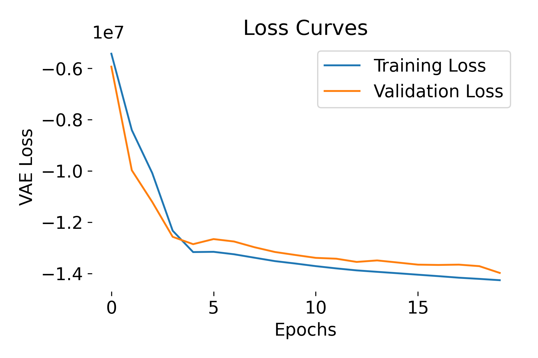
Loss curves of a VAE model trained on the MNIST dataset. The training and validation losses decrease over epochs, indicating that the model is learning and generalizing well. The negative ELBO loss is expected due to the negative reconstruction loss and non-negative KL divergence term.

The ELBO loss is negative but the model is learning, i.e., the loss is decreasing over epochs, and there is no divergence between training and validation losses. This behavior is expected and not a cause for concern. The expected log-likelihood term (reconstruction loss, BCE in our case) is usually negative, and its magnitude can be large. The KL divergence term is non-negative but often smaller in magnitude compared to the expected log-likelihood term. As a result, the ELBO, which is the difference between these two terms, can be negative. The key is, however, to ensure that the model is learning and the loss is decreasing over time.

To further validate the performance of out trained VAE model, let’s visualize some original and reconstructed images. To do so and as for the Autoencoder, we need to put the model in evaluation mode and iterate over some images without gradients (as we don’t want to update the model):

model.eval()
with torch.no_grad():
    images, _ = next(iter(test_loader))
    images = images.view(images.size(0), -1).to(device)
    recon_images, _, _ = model(images)
    recon_images = recon_images.view(-1, 28, 28).cpu()  # reshape for visualization

# plot the original and reconstructed images:
n = 5  # number of images to display
plt.figure(figsize=(10, 4))
for i in range(n):
    # Original image
    plt.subplot(2, n, i + 1)
    plt.imshow(images[i].view(28, 28).cpu().numpy(), cmap='gray')
    plt.title('Original')
    plt.axis('off')
    
    # Reconstructed image
    plt.subplot(2, n, i + 1 + n)
    plt.imshow(recon_images[i].numpy(), cmap='gray')
    plt.title('Reconstr.')
    plt.axis('off')
plt.show()

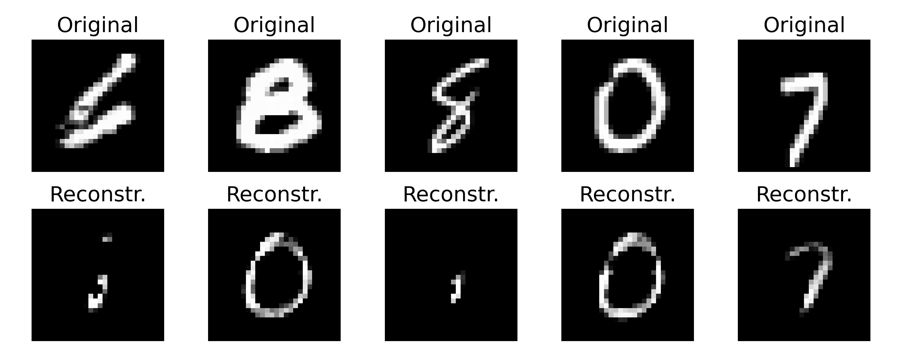
Example of original and reconstructed images by a VAE model trained on the MNIST dataset. Even though the training curves indicate a good training process, the reconstructed images show blurriness and incompleteness compared to the original images. This is a common characteristic of VAEs due to the KL divergence regularization. One can further tune the model or explore different architectures to improve the reconstruction quality.

At the end, let’s have a look how the VAE embeds the data into the latent space. In our case, we set the dimension of the latent space to 2, which allows us to visualize the latent space in a 2D plot. We again run the model in evaluation mode and iterate over the test data to get the latent representations:

latents = []
labels = []

with torch.no_grad():
    for images, lbls in test_loader:
        images = images.view(images.size(0), -1).to(device)
        mu, _ = model.encode(images)
        latents.append(mu.cpu().numpy())
        labels.append(lbls.cpu().numpy())

latents = np.concatenate(latents)
labels = np.concatenate(labels)

# plot the latent space with color-coded digits:
plt.figure(figsize=(8, 6))
scatter = plt.scatter(latents[:, 0], latents[:, 1], c=labels, cmap='tab10', alpha=0.7)
plt.colorbar(scatter, label='Digit Label')
plt.title('Latent Space Representation (color-coded by digits)')
plt.xlabel('Latent Dimension 1')
plt.ylabel('Latent Dimension 2')
plt.tight_layout()
plt.show()

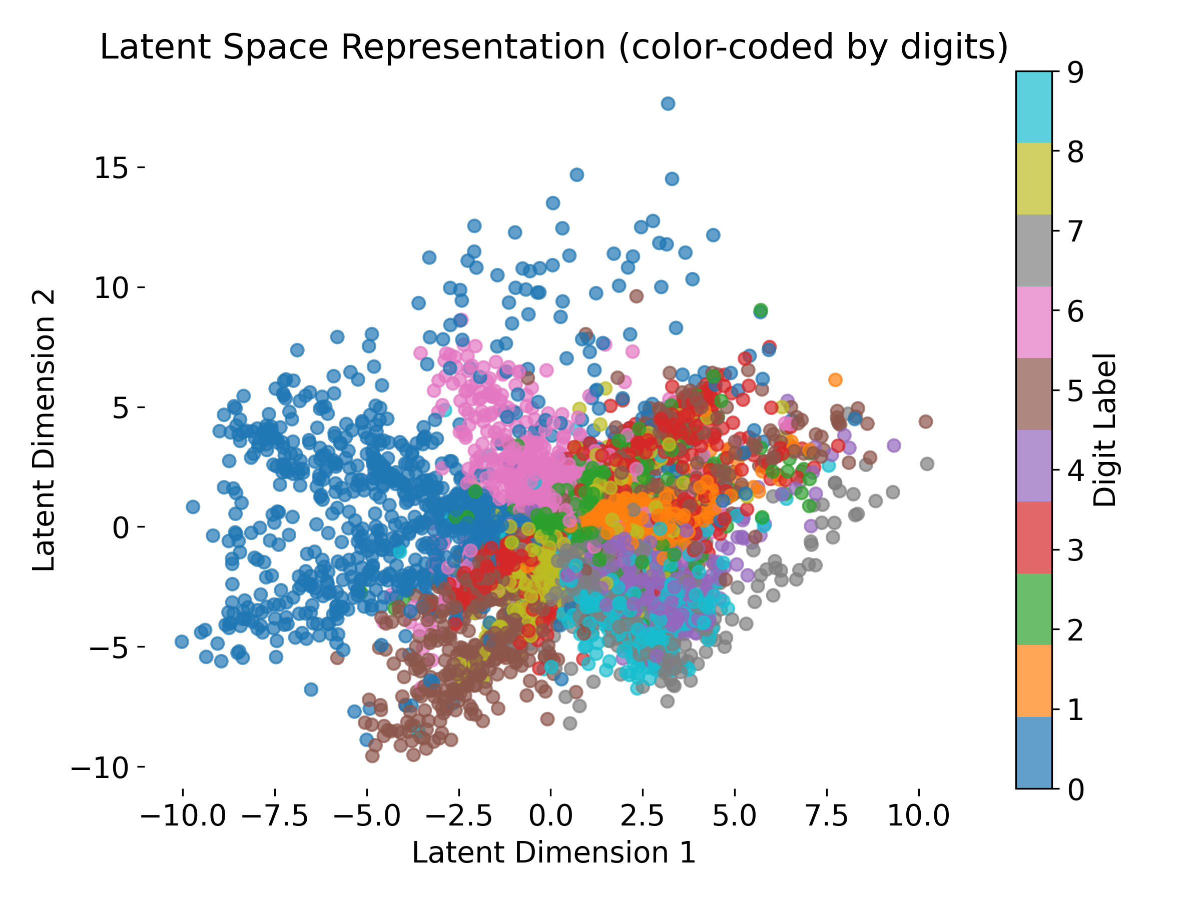
The VAE is able to embed the MNIST digits into a 2D latent space. Each point represents a digit, color-coded by its label. The latent space shows a (kind of) structured distribution, with similar digits clustered together. A well structured latent space enables meaningful interpolation and generation of new samples. In neuroscience, such latent representations can help uncover underlying patterns in neural data.

$\beta$-VAE

Now let’s see, how both the model architecture and the outcome change when we implement a $\beta$-VAE.

In a $\beta$-VAE, we often reduce the network complexity (i.e., number of layers or neurons) for two main reasons:

1. Increased regularization with $\beta$-term: In $\beta$-VAE, we introduce a higher weight ($\beta \gt 1$) on the KL term in the loss function. This means that the model is penalized more heavily for deviations from the prior distribution (usually a Gaussian) in the latent space. This stronger regularization encourages the model to disentangle the latent representations, often by sacrificing some reconstruction accuracy in favor of enforcing a structured latent space. By reducing the number of layers, we reduce the model’s capacity, which aligns with the higher regularization: we prevent the model from overfitting or becoming overly complex, which would counteract the disentangling effect we’re trying to achieve with $\beta$.
2. Simplicity to facilitate disentangling: Disentangling means encouraging each latent dimension to represent a distinct, independent factor of variation in the data. Simpler architectures, with fewer layers and parameters, tend to have a better inductive bias for disentangling. When the model has fewer layers, it’s often forced to represent the data in a more compressed and disentangled way because it doesn’t have the extra capacity to represent redundant or overlapping features. This encourages each latent dimension to capture separate, interpretable aspects of the data.

In practice, many $\beta$-VAE implementations thus use simpler architectures than standard VAEs. Therefore, let’s update our model architecture accordingly (we simply take out one fully connected layer from the encoder and decoder):

class BetaVAE(nn.Module):
    def __init__(self, input_dim, latent_dim, beta=1.0):
        super(BetaVAE, self).__init__()
        self.beta = beta
        
        # encoder:
        self.fc1 = nn.Linear(input_dim, 128)
        self.fc2_mu = nn.Linear(128, latent_dim)
        self.fc2_logvar = nn.Linear(128, latent_dim)
        
        # decoder:
        self.fc3 = nn.Linear(latent_dim, 128)
        self.fc4 = nn.Linear(128, input_dim)

    def encode(self, x):
        h1 = torch.relu(self.fc1(x))
        return self.fc2_mu(h1), self.fc2_logvar(h1)

    def reparameterize(self, mu, logvar):
        std = torch.exp(0.5 * logvar)
        eps = torch.randn_like(std)
        return mu + eps * std

    def decode(self, z):
        h3 = torch.relu(self.fc3(z))
        return torch.sigmoid(self.fc4(h3))

    def forward(self, x):
        mu, logvar = self.encode(x)
        z = self.reparameterize(mu, logvar)
        return self.decode(z), mu, logvar

We need to redefine the loss function to include the $\beta$-term:

# define loss function with beta parameter:
def beta_vae_loss(recon_x, x, mu, logvar, beta=1.0):
    # Binary Cross-Entropy (Reconstruction) loss
    recon_loss = nn.functional.binary_cross_entropy(recon_x, x, reduction='sum')
    
    # KL Divergence with beta scaling
    kld_loss = -0.5 * torch.sum(1 + logvar - mu.pow(2) - logvar.exp())
    
    # Total loss with beta parameter
    return recon_loss + beta * kld_loss

Initializing the model works as before, we just need to additionally hand-over the $\beta$ parameter:

# model:
input_dim = 784  # Example for MNIST flattened input
latent_dim = 20
beta = 20  # Experiment with different values (e.g., 0.1, 0.5, 2, 4, 10)
model = BetaVAE(input_dim, latent_dim, beta=beta)

The rest of the training loop and validation is the same as for the standard VAE.

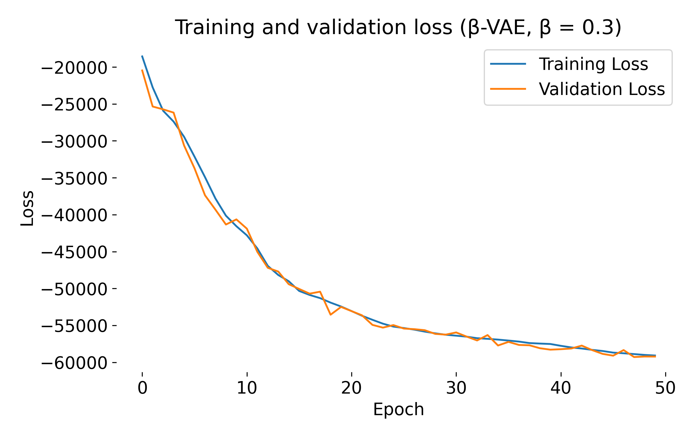
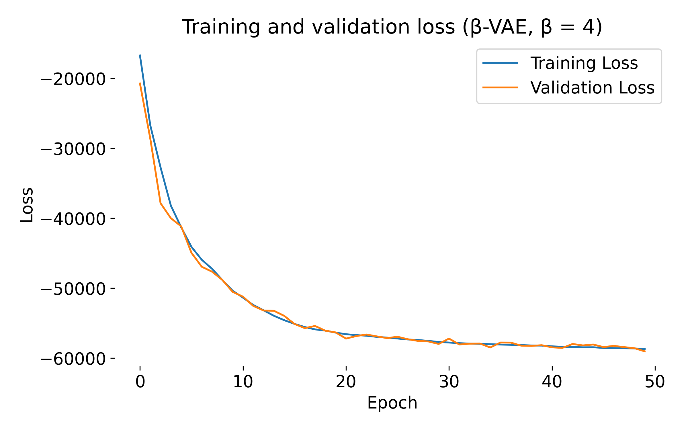
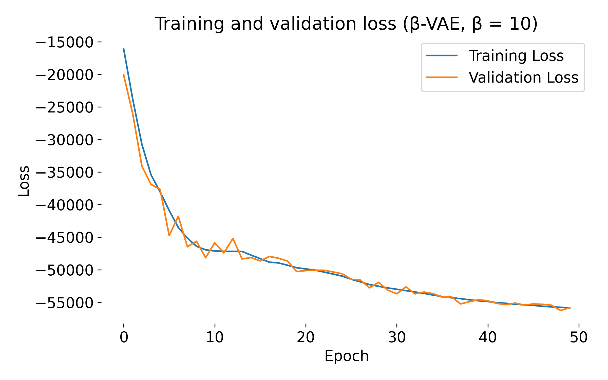
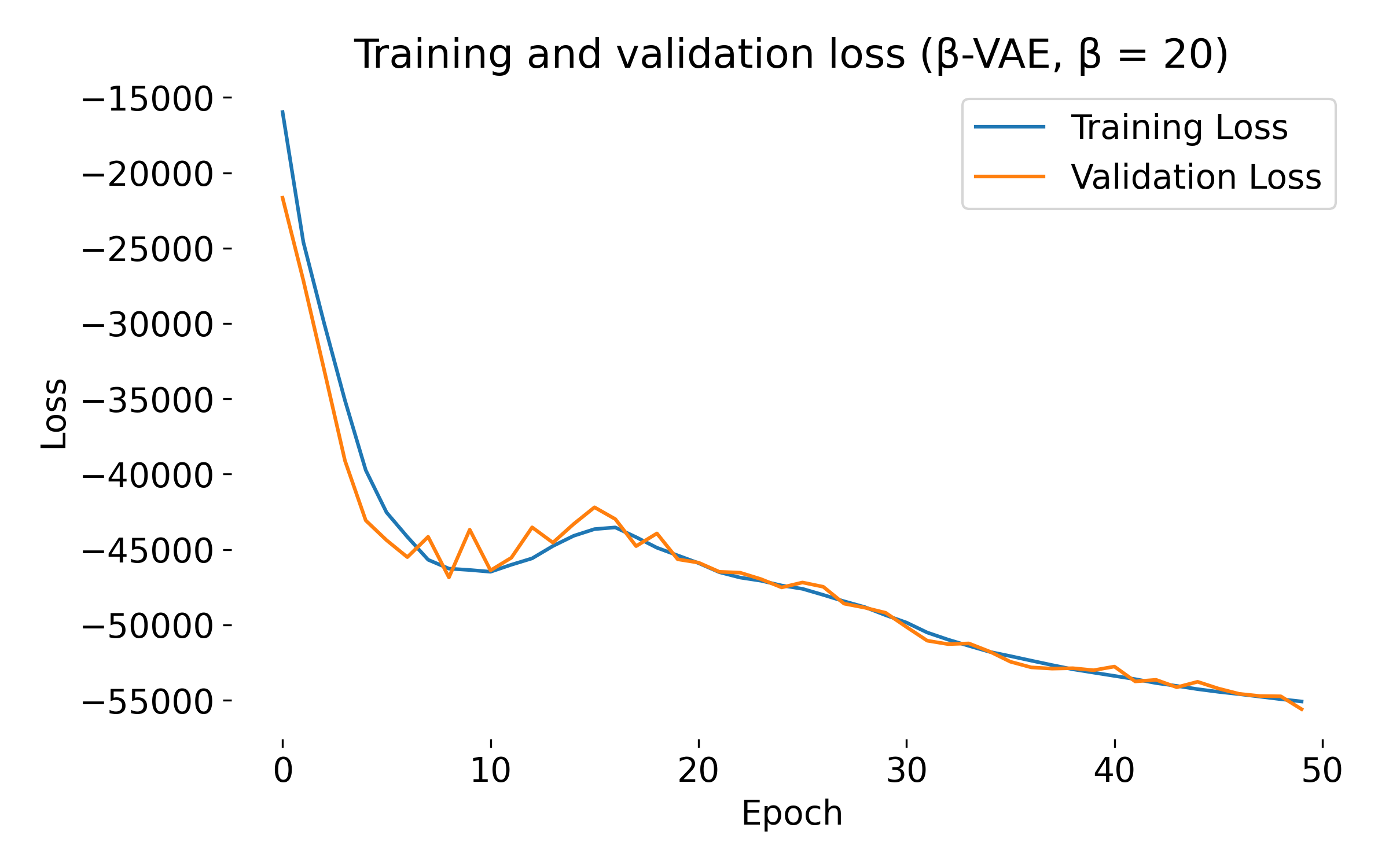
Loss curves of a $\beta$-VAE model trained on the MNIST dataset with different $\beta$ values. The training and validation losses decrease over epochs, indicating that the model is learning and generalizing well. At first glance, we see no significant difference in the loss curves for different $\beta$ values, except for $\beta=20$, where both training and validation loss show an usual dip at the beginning. This behavior might indicate that the model is struggling to balance the reconstruction and KL divergence terms, which can be further investigated by tuning the model.

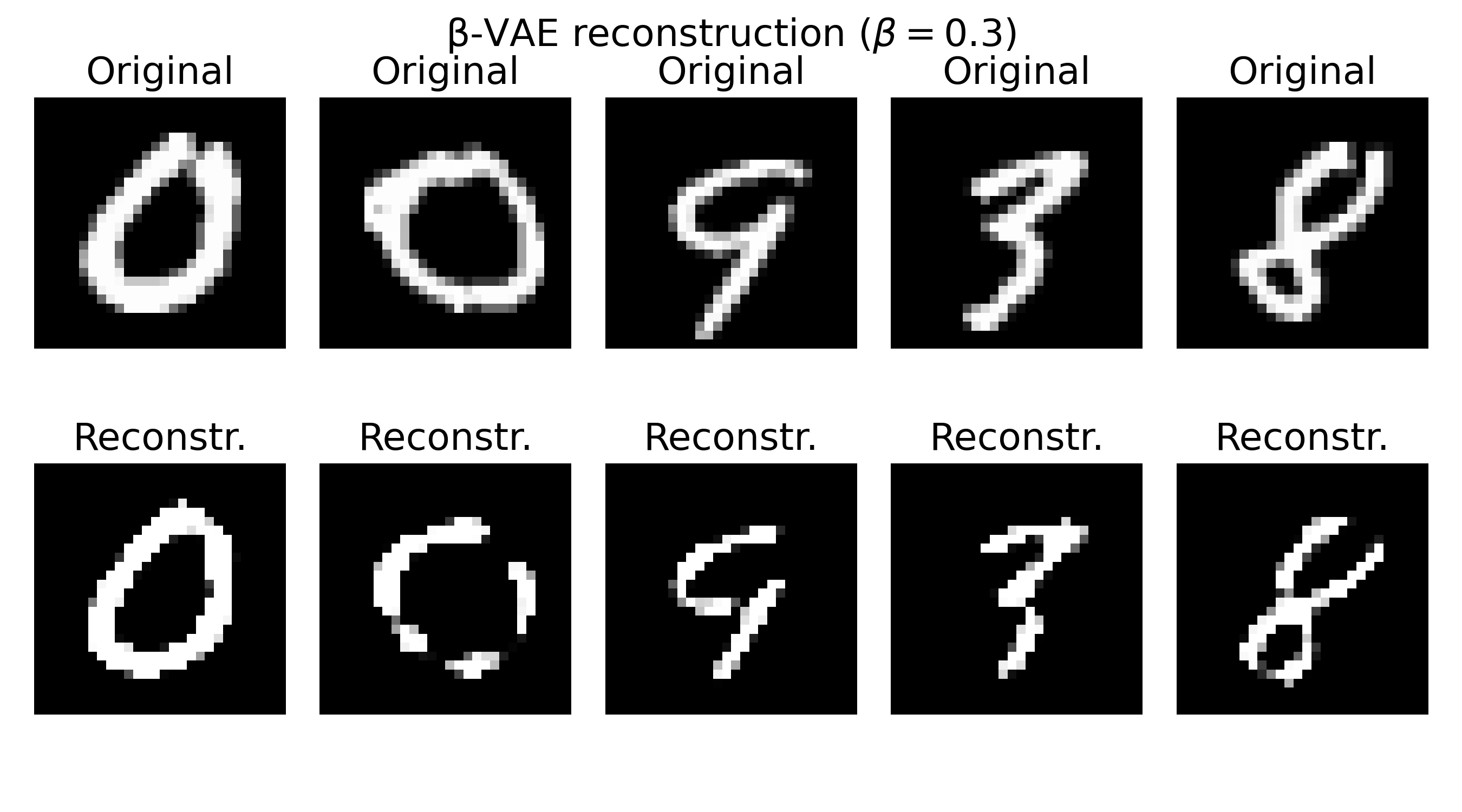
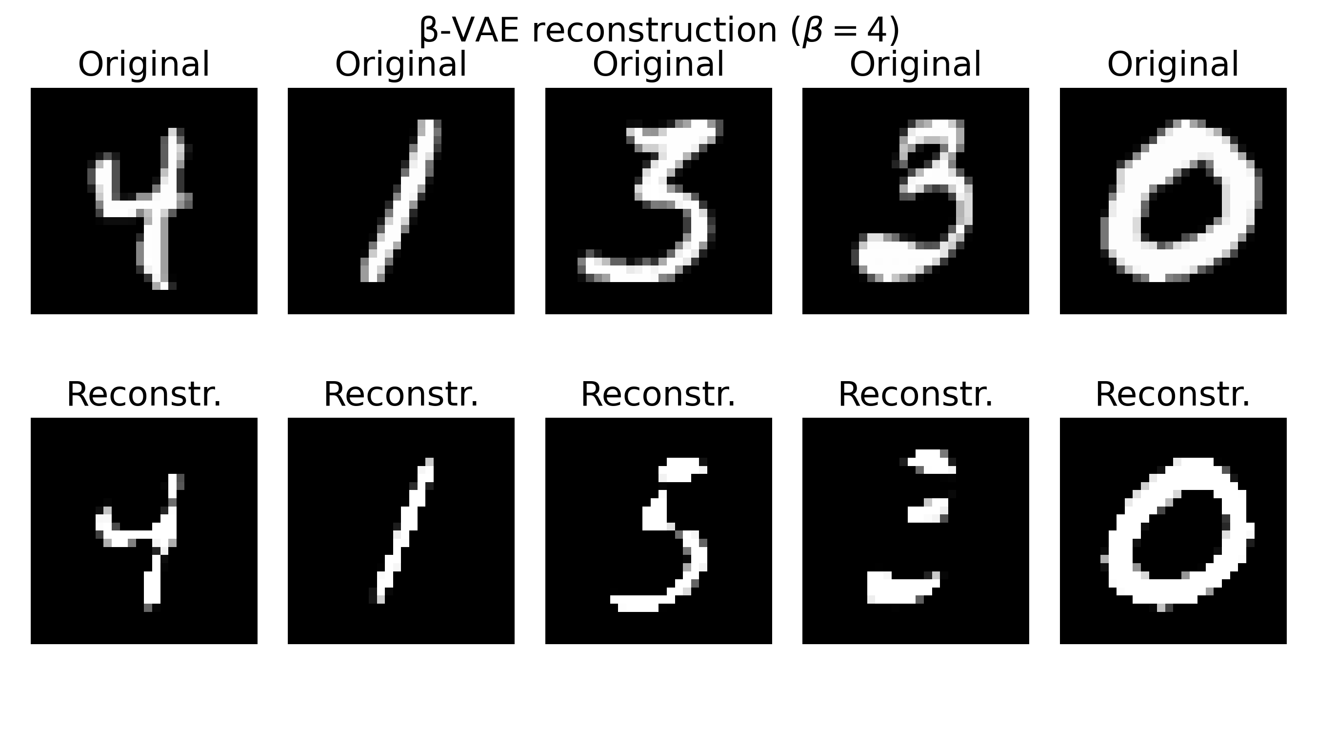
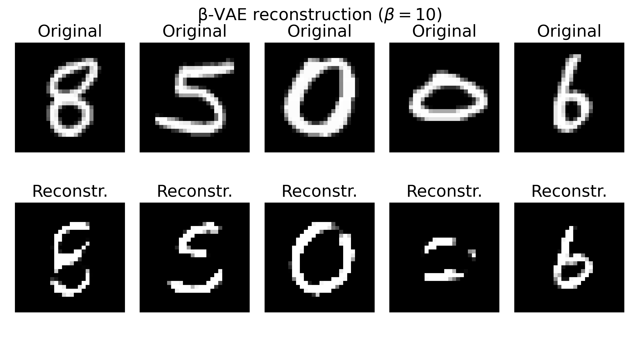
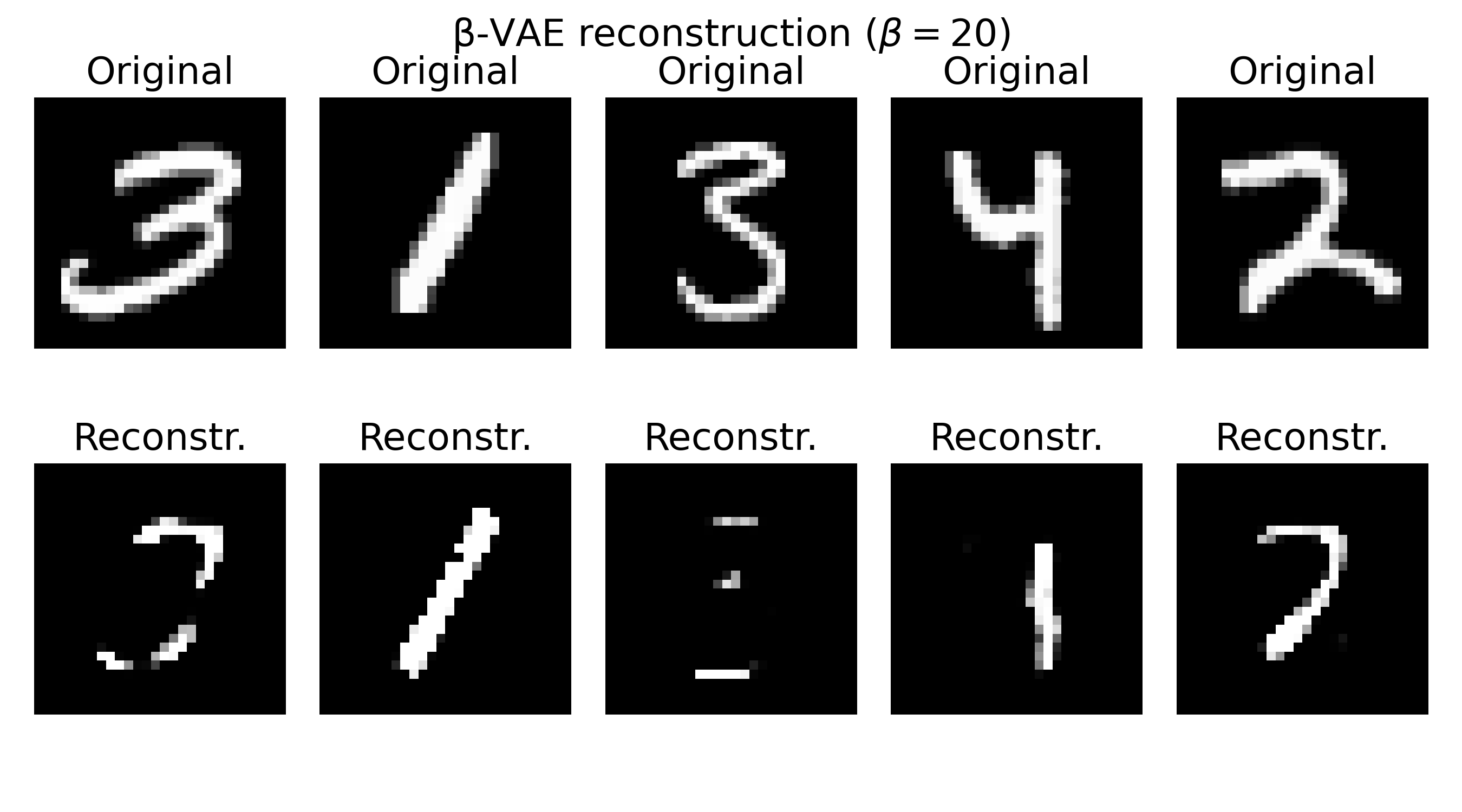
Sample reconstructions of a $\beta$-VAE model trained on the MNIST dataset with different $\beta$ values. The reconstructions show varying levels of blurriness and incompleteness, depending on the choice of $\beta$. Lower $\beta$ values (e.g., $\beta=0.3$) prioritize reconstruction quality, leading to sharper but less structured reconstructions. Higher $\beta$ values (e.g., $\beta=20$) prioritize the KL divergence term, resulting in more structured but blurrier reconstructions. The choice of $\beta$ should be tuned based on the desired balance between reconstruction quality and latent space regularization.

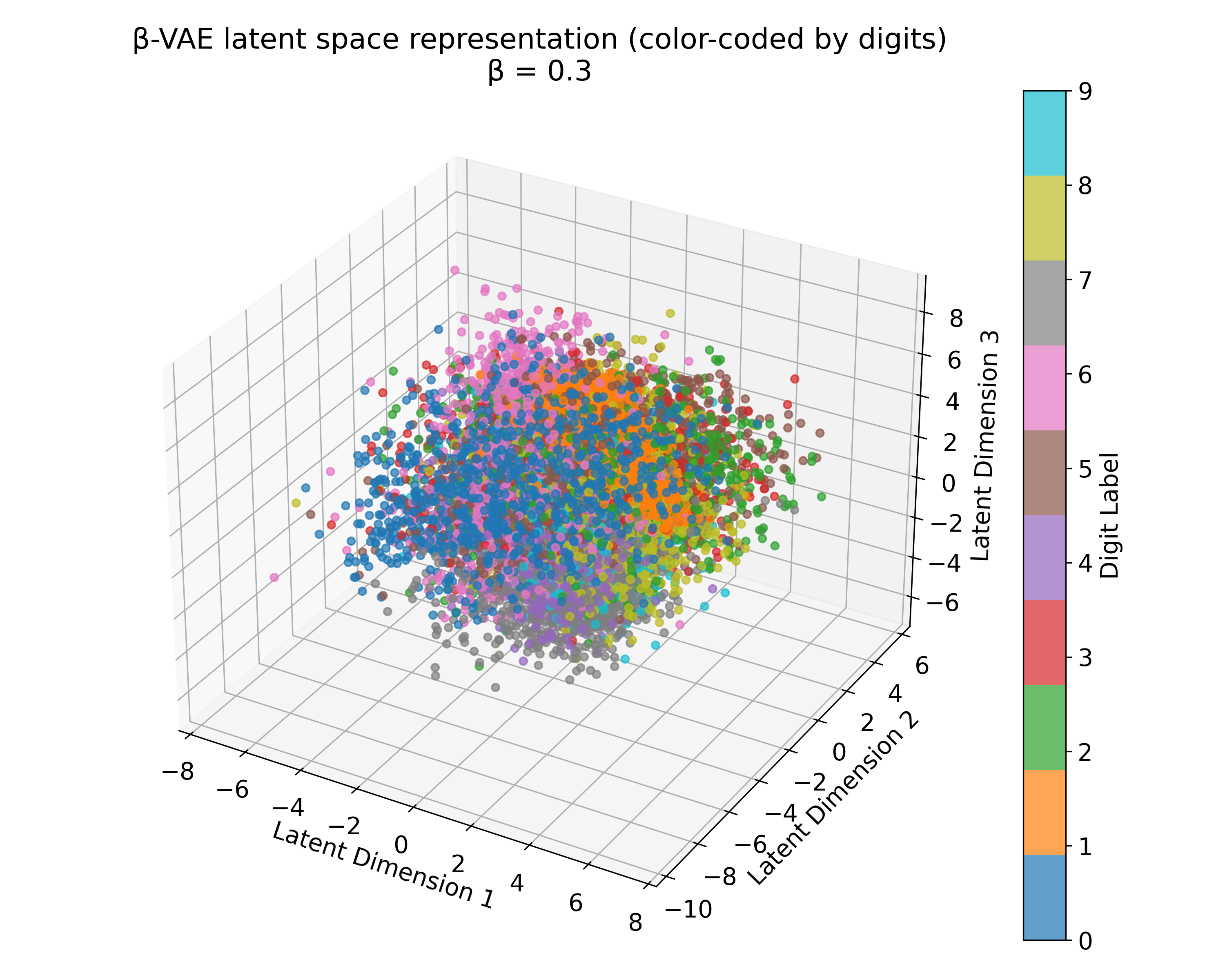
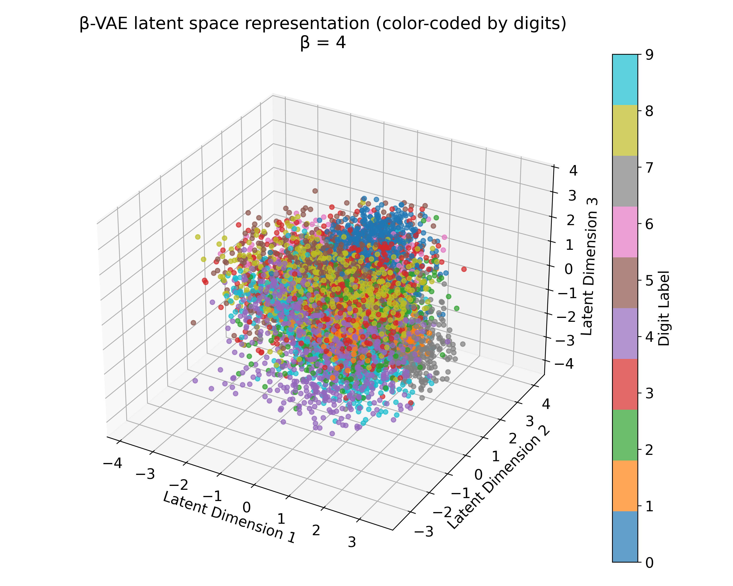
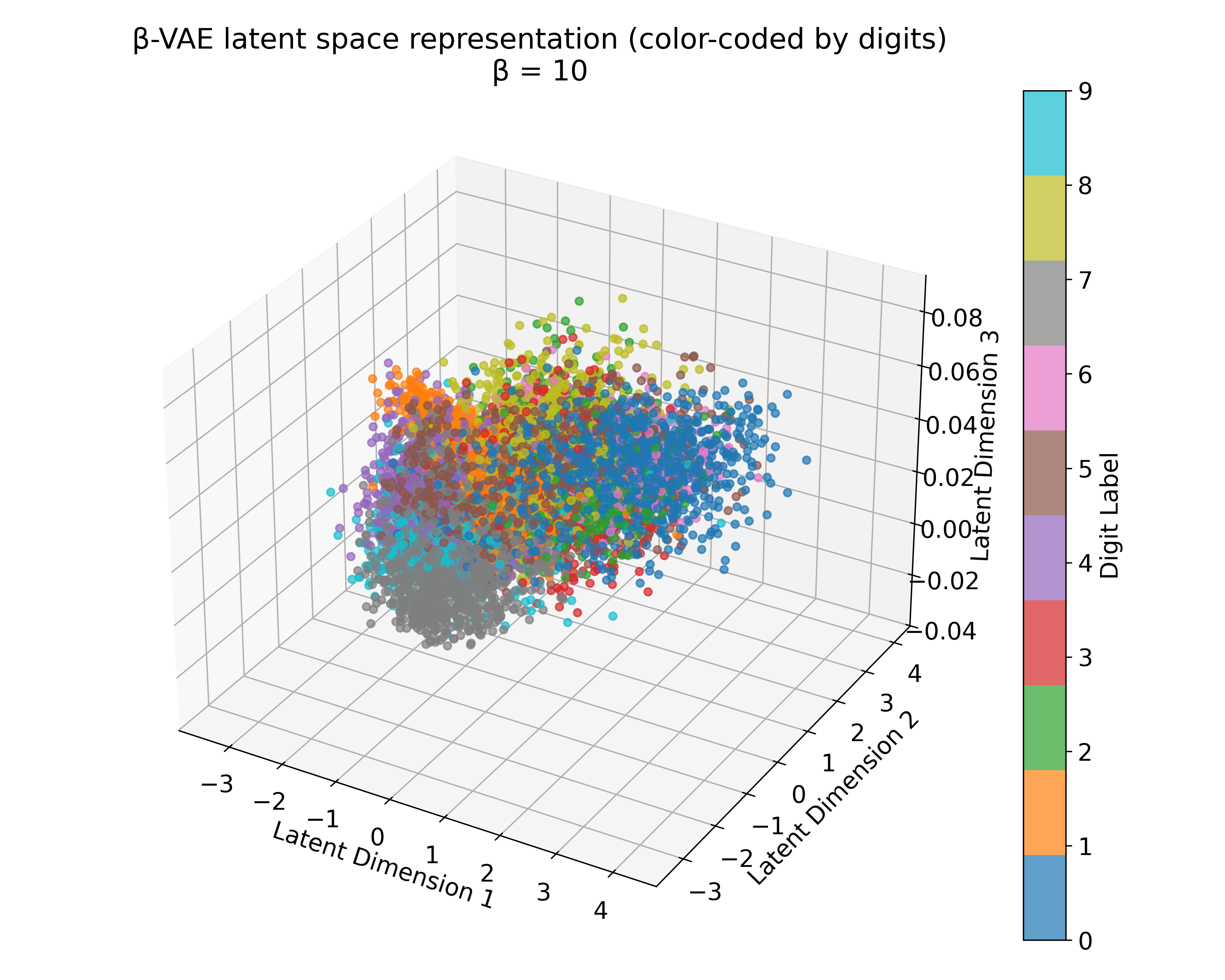
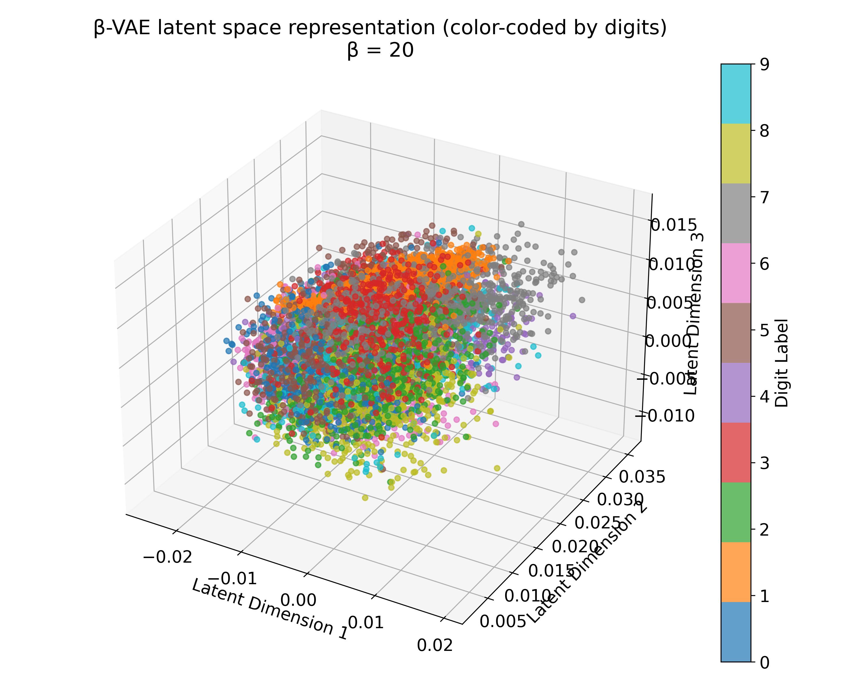
Latent space representations of a $\beta$-VAE model trained on the MNIST dataset with different $\beta$ values. The 3D plots (we trained the model with latent_dim=3) show the distribution of the digits embedded in the latent space. Higher $\beta$ values lead to more structured and separated clusters, indicating a more disentangled latent space. However, this doesn’t scale linearly with $\beta$, and the choice of $\beta$ should be tuned based on the desired balance between reconstruction quality and latent space regularization. A too high $\beta$ value can lead to over-regularization and loss of reconstruction quality due to the strong emphasis on the KL divergence term.

Exercise

In the exercise, you will implement a VAE to embed neural and behavior data into a low-dimensional latent space. You will train the VAE model on the data and visualize the latent space representations. You will also use the trained VAE model to make behavior predictions based on neural activity. You will learn how to fine-tune the model in order to balance the reconstruction quality and the regularization of the latent space.

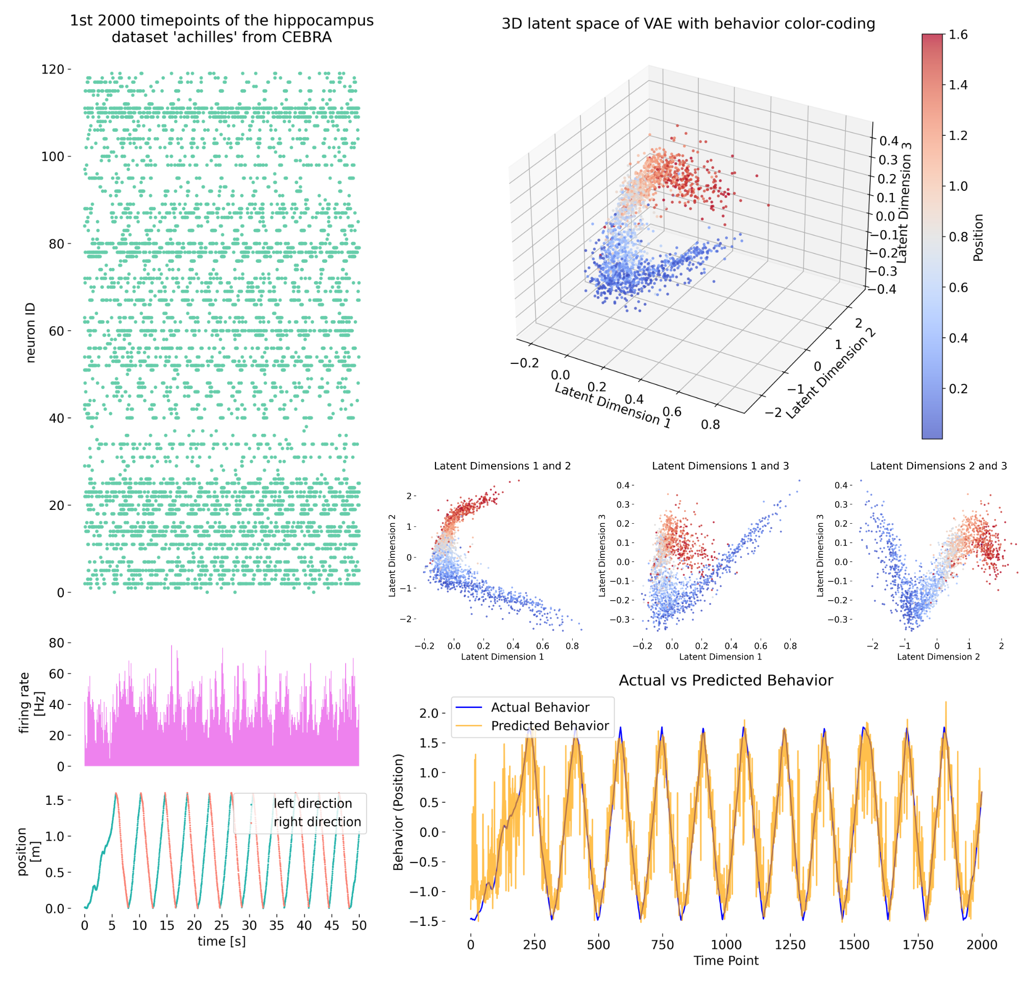
In the exercise, we will embed the high-dimensional neural and behavior data into a low-dimensional latent space using a VAE. The latent space representations will help us visualize the data in a structured and interpretable way, facilitating further analysis and insights into the neural-behavior relationship. We will also use the trained VAE model to make behavior predictions based on neural activity.

Access the exercise notebook here: