Excurse: Artificial Neural Networks (ANN)

This chapter provides a brief introduction on artificial neural networks, providing supporting information to the neural networks used throughout this course.

Overview

Artificial neural networks (ANN) are computational models inspired by the human brain, designed to recognize patterns and learn from data. ANNs consist of interconnected layers of nodes, called neurons, that transform input data through a series of mathematical operations. Unlike traditional algorithms, ANNs can learn complex, non-linear relationships within data, making them especially effective in tasks involving images, sound, text – and dimensionality reduction.

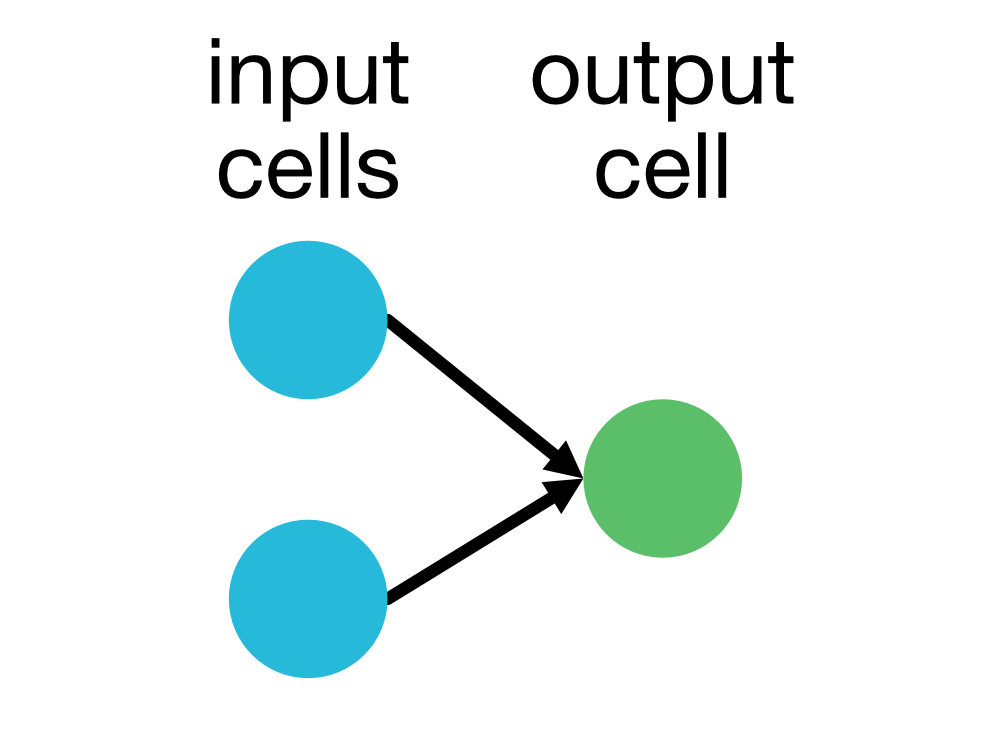The perceptron, depicted here, is the simplest form of a neural network, consisting of a single input and output layer.

Basic structure of an ANN

The architecture of a simple feedforward neural network, one of the most common types of ANNs, consists of the following components:

1. Input Layer:
   • The input layer receives the initial data, which could be images, text, or numerical data, and passes it to the network.
   • Each neuron in this layer represents a feature or attribute of the input data.
2. Hidden Layers:
   • Hidden layers lie between the input and output layers and perform complex transformations on the data.
   • The network can have one or more hidden layers, each comprising a series of neurons that apply transformations to the inputs from the previous layer. These transformations are made possible by weights and biases (parameters that the network adjusts during training) and activation functions (which introduce non-linearity into the network, allowing it to learn complex patterns).
3. Output Layer:
   • The output layer produces the final prediction or decision based on the transformed input.
   • In classification tasks, the output is often converted into probabilities using functions like softmax (for multi-class classification) or sigmoid (for binary classification). The number of neurons in this layer depends on the number of target classes or outputs.

Structure of an artificial neuron

An artificial neuron, inspired by biological neurons, is a computational unit that processes inputs, applies weights, and produces an output. The main components are:

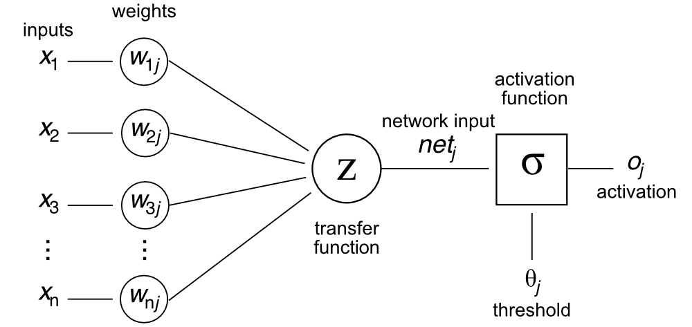Diagram of an artificial neuron in an artificial neural network. The neuron receives inputs $x_1, x_2, …, x_n$, multiplies them by corresponding weights $w_1, w_2, …, w_n$, and adds a bias term $b$. The weighted sum is passed through an activation function $\sigma$ to produce the neuron’s output $o$ (also denoted as $y$, see below). Adapted from Wikimedia Commonsꜛ (license: CC BY-SA 3.0).

1. Inputs $x_1, x_2, …, x_n$:
   • These are the features or signals that the neuron receives. In a neural network, each neuron typically receives inputs from neurons in the previous layer, or in the case of the first layer, from the raw data features.
   • Each input $x_i$ has an associated weight $w_i$ that determines the influence of that input on the neuron’s output.
2. Weights $w_1, w_2, …, w_n$:
   • Weights are adjustable parameters that control the importance of each input.
   • The neuron will “learn” appropriate values for these weights during the training process to minimize error.
   • Initially, weights are often set randomly and then adjusted as the model is trained.
3. Weighted sum $z$:

   • The neuron computes a weighted sum of its inputs. Mathematically, this can be represented as:

     \[z = \sum_{i=1}^{n} w_i x_i + b\]
   • Here, $z$ is the pre-activation output (also called the net input), and $b$ is the bias term.
   • The bias is an additional parameter that allows the activation function to shift horizontally, enabling the neuron to learn more complex functions.
4. Activation function $\sigma(z)$:
   • The weighted sum $z$ is passed through an activation function $\sigma$.
   • The activation function introduces non-linearity, allowing the neuron to capture complex patterns in the data.
   • Common activation functions include sigmoid, ReLU (Rectified Linear Unit), and tanh. Each has different properties and is suited for different types of tasks.
5. Output $o_j$:
   • The result after applying the activation function is the neuron’s output, which is passed to neurons in the next layer or, in the case of the output layer, used to make a final prediction.

The operation of an artificial neuron can be summarized with the following equation:

\[o_j = y = \sigma\left( \sum_{i=1}^{n} w_i x_i + b \right)\]

where:

• $y$ is the neuron’s output,
• $\sigma$ is the activation function,
• $w_i$ are the weights for each input $x_i$,
• $b$ is the bias.

Thus, the workflow of an artificial neuron involves:

1. Input processing: Each input $x_i$ is multiplied by its corresponding weight $w_i$.
2. Summation: All weighted inputs are summed, and the bias $b$ is added to the sum.
3. Activation: The weighted sum is passed through the activation function to produce the neuron’s output.
4. Output propagation: The output is sent to other neurons in the next layer or, if the neuron is in the output layer, is used as part of the final model prediction.

This simple yet powerful computation is the basis for how neurons process information in an artificial neural network. By adjusting the weights and biases, the neuron “learns” to generate outputs that minimize prediction errors, thereby allowing the network to learn complex patterns in the data.

Forward propagation in ANNs

The process of feeding input data through the layers of a neural network to produce an output is known as forward propagation. Each neuron in a layer computes a weighted sum of its inputs, adds a bias term, and passes the result through an activation function. This process is repeated layer by layer until the network produces an output.

Mathematically, for a given layer $l$:

1. Each neuron receives the outputs (activations) from the previous layer, $\mathbf{h}^{(l-1)}$.
2. It applies a linear transformation using weights $\mathbf{W}^{(l)}$ and biases $\mathbf{b}^{(l)}$.

3. Finally, it applies an activation function $\sigma$ to introduce non-linearity:

   \[\mathbf{h}^{(l)} = \sigma\left(\mathbf{W}^{(l)} \mathbf{h}^{(l-1)} + \mathbf{b}^{(l)}\right)\]

In this way, the network transforms the data through successive layers, enabling it to model complex relationships.

Training neural networks

The power of neural networks lies in their ability to learn from data. During training, a neural network iteratively adjusts its parameters (weights and biases) to minimize the difference between its predictions and the actual outputs. This process is driven by two key components: the loss function and backpropagation.

Loss function

The loss function quantifies the difference between the network’s predictions and the true values. The choice of the loss function depends on the specific task:

• For regression tasks, the mean squared error (MSE) is commonly used:

  \[\text{MSE} = \frac{1}{n} \sum_{i=1}^{n} (y_i - \hat{y}_i)^2\]

  where $y_i$ are the true values and $\hat{y}_i$ are the predicted values. $$

• For classification tasks, the cross-entropy loss is widely applied:

  \[\text{Cross-Entropy Loss} = -\sum_{i=1}^{n} y_i \log(\hat{y}_i)\]

The goal of training is to minimize this loss function, effectively improving the network’s accuracy in making predictions.

Backpropagation and gradient descent

To optimize the network parameters, ANNs use an algorithm called backpropagation in conjunction with gradient descent (or its variants). Backpropagation works by computing the gradient of the loss function with respect to each parameter, which tells the network how to adjust its weights and biases to reduce the loss.

Steps in Backpropagation:

1. Compute the loss: Measure the error between the network’s output and the true output using the loss function.
2. Calculate gradients: Use the chain rule to compute the gradient of the loss function with respect to each parameter.
3. Update parameters: Adjust the parameters by moving them in the opposite direction of the gradient to minimize the loss. This is done using an optimization algorithm, commonly stochastic gradient descent (SGD) or Adam (a variant of SGD).

The update rule for each weight $w$ can be written as:

\[w_{\text{new}} = w_{\text{old}} - \eta \cdot \frac{\partial L}{\partial w}\]

where $\eta$ is the learning rate, a hyperparameter that controls the step size of each update.

This iterative process of forward propagation, loss calculation, backpropagation, and parameter updates continues over many epochs (complete passes through the training data) until the model reaches a satisfactory level of accuracy.

Types of ANN

There are several types of neural networks, each suited to different types of data and tasks.

Perceptrons (P)

Perceptrons are the simplest form of neural networks, consisting of an input layer and an output layer. They are used for binary classification tasks and are the building blocks of more complex networks.

Perceptrons are the simplest form of neural networks, consisting of an input layer and an output layer. It is used for binary classification tasks.

Hopfield Networks (HN) and Boltzmann Machines (BM)

Hopfield networks and Boltzmann machines are used for associative memory and optimization problems, respectively. They are often applied in unsupervised learning tasks. In a Hopfield network, neurons are fully connected, while Boltzmann machines have both input and (probabilistic) hidden neurons. Input cells are output as soon as each hidden cell updates its state (during training, BMs / HNs update cells sequentially and not in parallel).

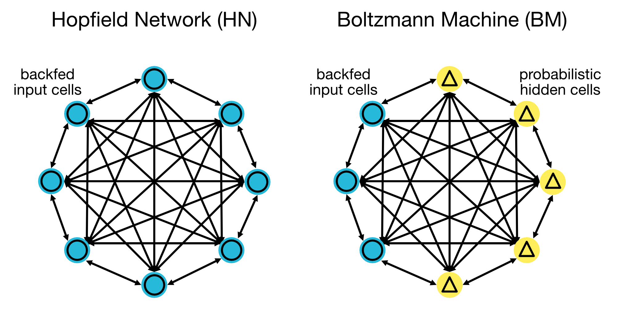Architecture of Hopfield Networks (HN, left) and Boltzmann Machines (BM, right). Hopfield networks are used for associative memory, while Boltzmann machines are used for optimization problems.

Feedforward Neural Networks (FNN)

In FNNs, information moves only in one direction — from the input layer to the output layer. These networks are simple and well-suited to structured data and straightforward tasks.

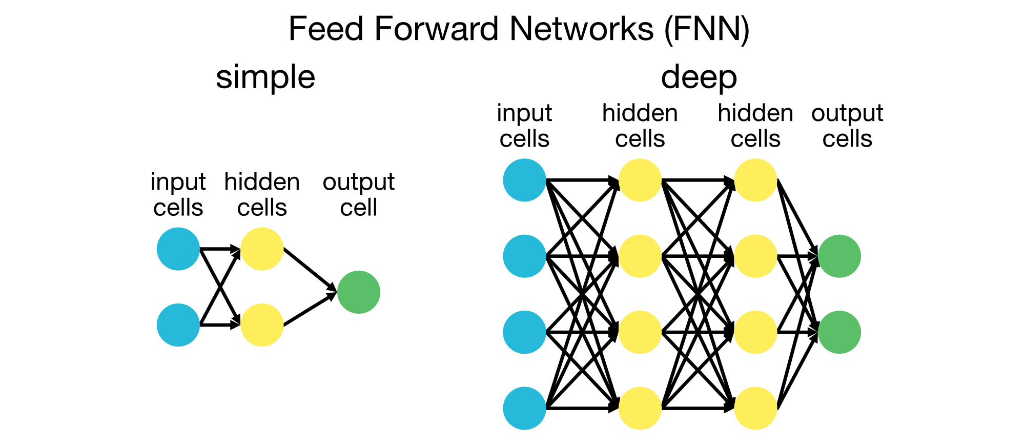
A simple (left) and deep (right) Feedforward Neural Network (FNN). Feedforward neural networks are used for structured data and straightforward tasks.

Convolutional Neural Networks (CNN)

CNNs are specifically designed for processing grid-like data structures, such as images. They use convolutional layers to detect spatial hierarchies in images, making them highly effective for image classification, object detection, and more.

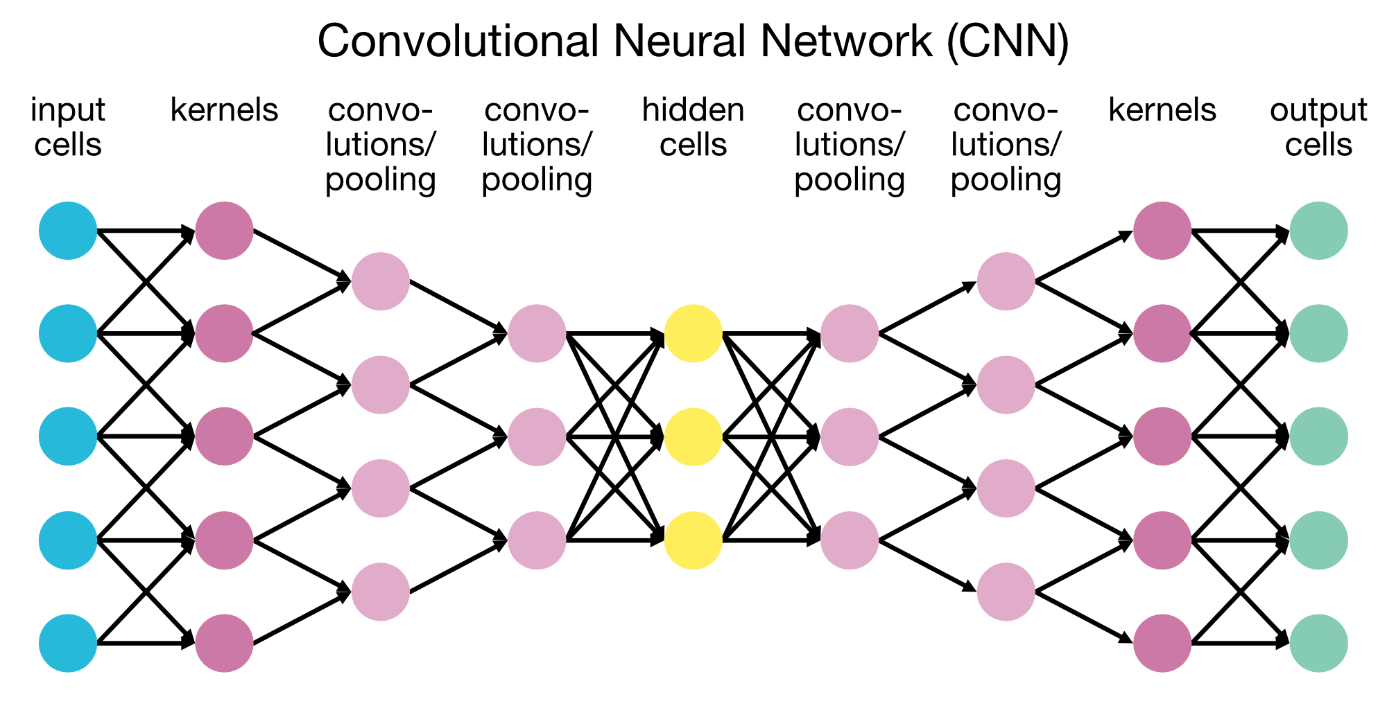
Convolutional Neural Networks (CNNs) are designed for processing grid-like data structures, such as images. They use convolutional layers to detect spatial hierarchies in images. This specific architecture consists of an encoder and a decoder part, which are used for image segmentation tasks. For simple image classification tasks, the decoder part can be omitted.

Recurrent Neural Networks (RNN)

RNNs are designed to handle sequential data, such as time series and text. They have connections that loop back, enabling them to maintain a memory of previous inputs, making them suitable for tasks like language modeling, speech recognition, and machine translation.

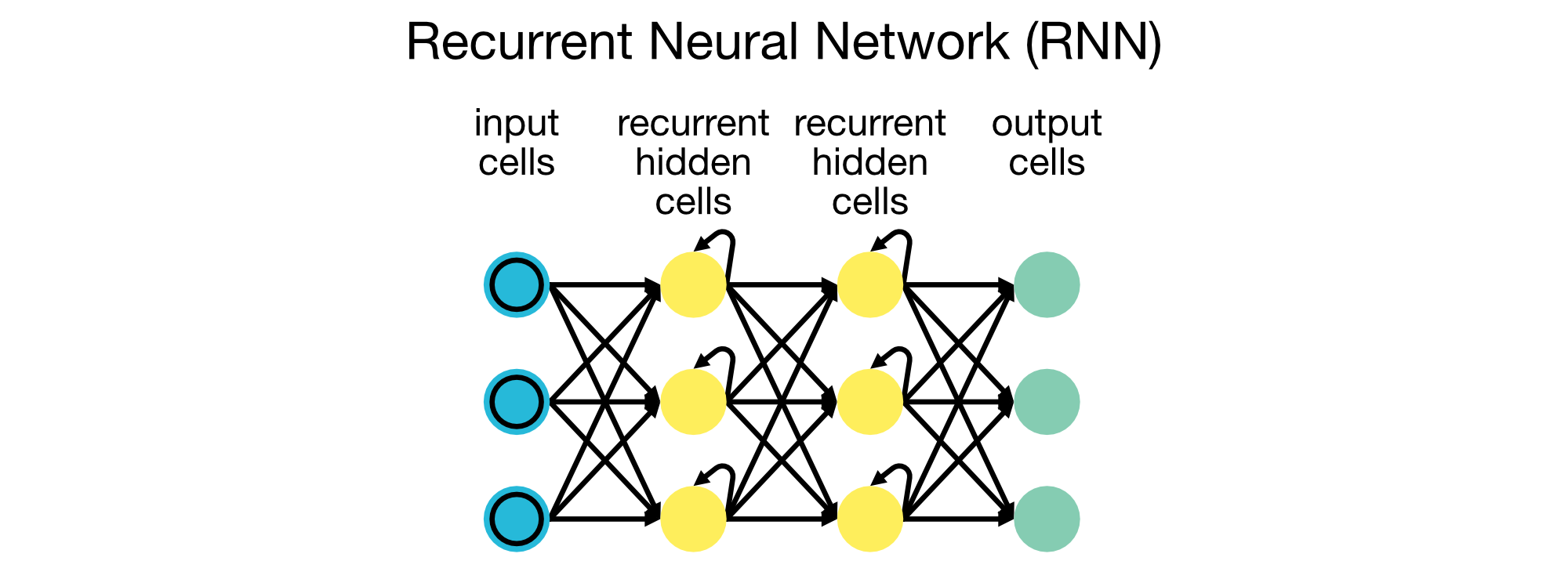
Recurrent Neural Networks (RNNs) are designed for sequential data, such as time series and text. They have connections that loop back, enabling them to maintain a memory of previous inputs.

Autoencoders (AE)

Autoencoders are used for unsupervised learning, aiming to compress and reconstruct input data. They are widely used in dimensionality reduction, anomaly detection, and data denoising.

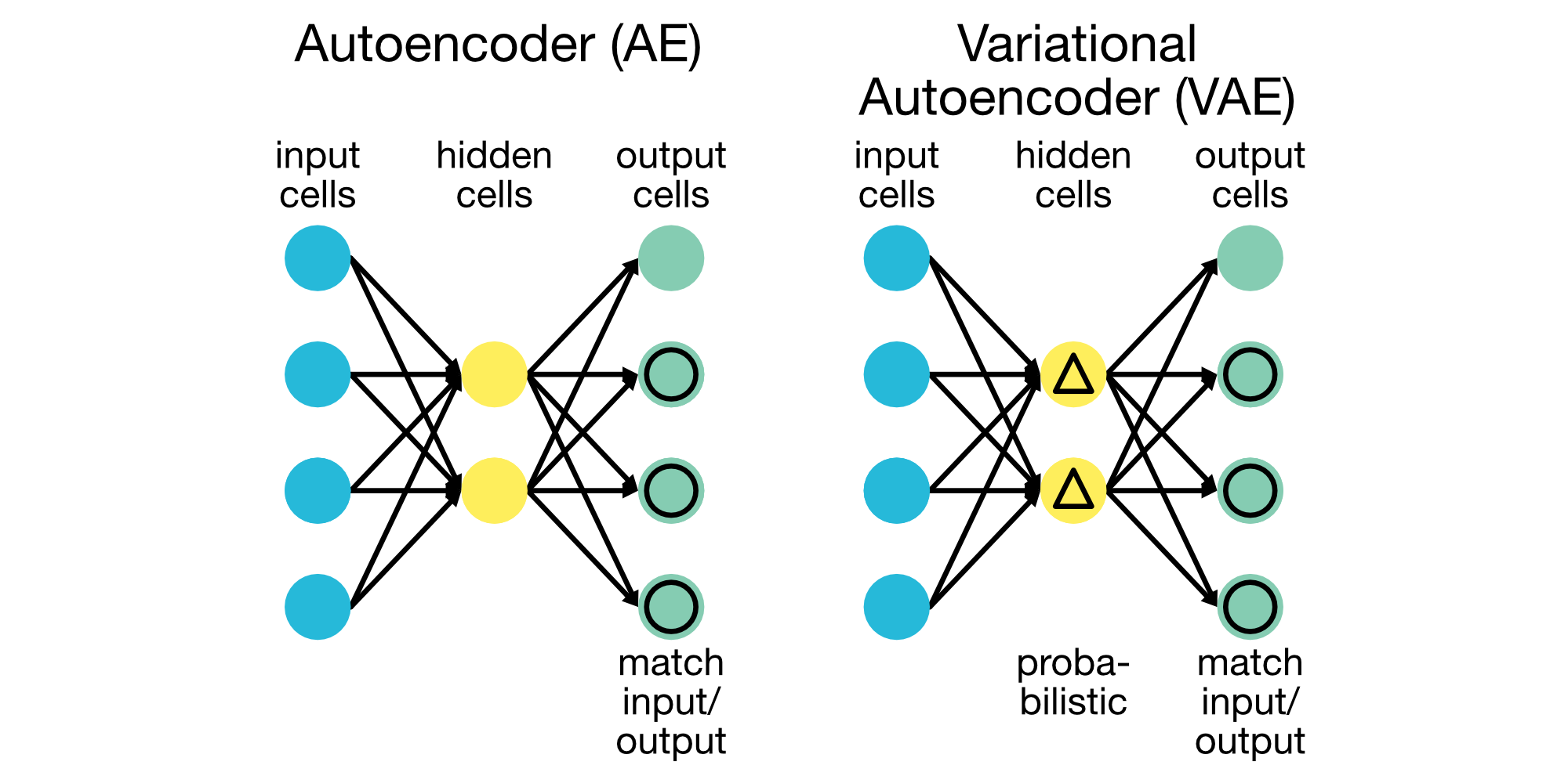
A simple default Autoencoder (AE, left) and a Variational Autoencoder (VAE, right). Autoencoders are used for unsupervised learning tasks, such as dimensionality reduction and data denoising.

Generative Adversarial Networks (GAN)

GANs consist of two networks, a generator and a discriminator, that compete against each other. GANs are used for generating new data samples, often indistinguishable from real data, making them useful for applications like image generation and synthetic data creation.

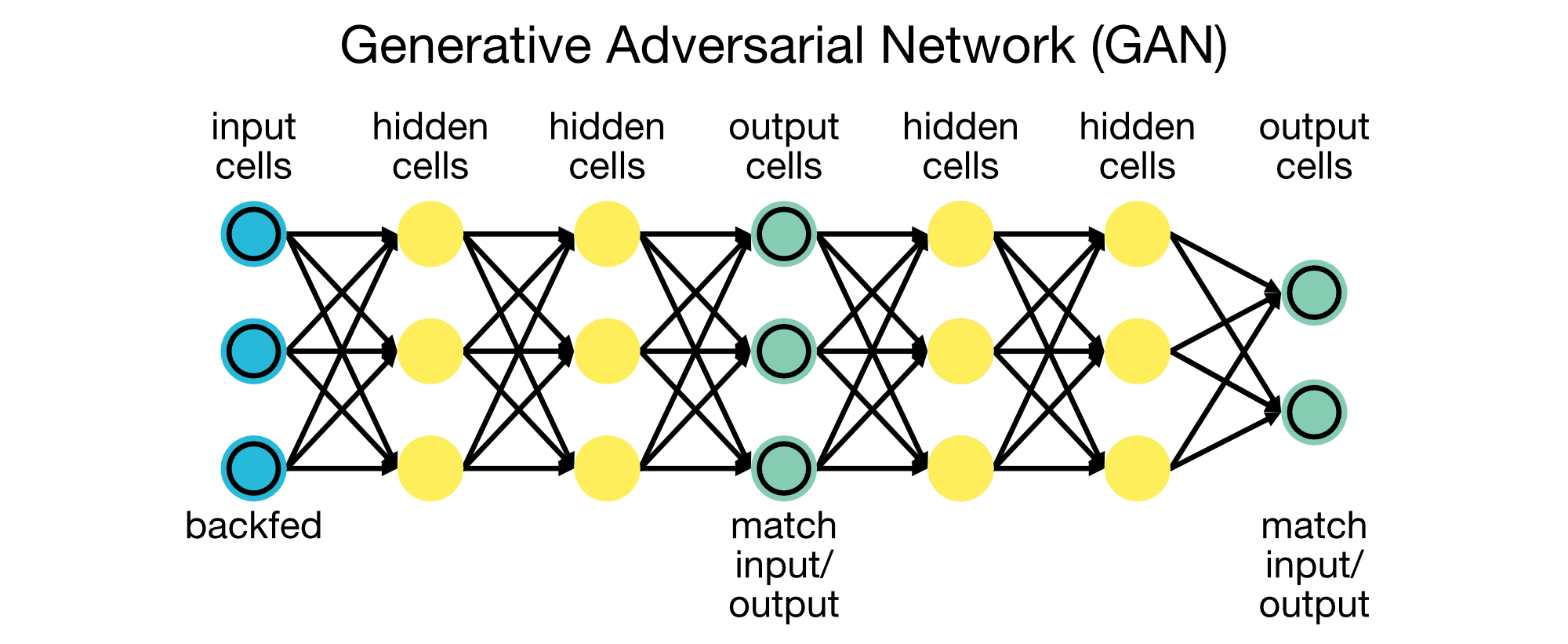
Generative Adversarial Networks (GANs) consist of a generator and a discriminator that compete against each other. GANs are used for generating new data samples, often indistinguishable from real data.

Key challenges in neural network training

Training neural networks, especially deep networks, comes with challenges that require careful handling.

Overfitting

When a model learns the noise in the training data rather than the true underlying patterns, it overfits and performs poorly on new data. Techniques such as regularization (e.g., L2 regularization, dropout) and early stopping help mitigate overfitting.

Vanishing and exploding gradients

In deep networks, gradients can become very small or excessively large during backpropagation, causing issues in parameter updates. Techniques such as ReLU activation functions, batch normalization, and weight initialization (e.g., Xavier, He) help alleviate these problems.

Hyperparameter tuning

Parameters like the learning rate, number of hidden layers, activation functions, and batch size need careful tuning for optimal performance. Grid search, random search, and advanced techniques like Bayesian optimization are used for hyperparameter tuning.

Python examples

Here are some examples using PyTorch to construct simple neural networks for image recognition tasks. Before running these examples, make sure PyTorch and torchvision (for loading datasets) are installed:

pip install torch torchvision

Example 1: Simple Feedforward Neural Network (FNN) for MNIST

This example shows a simple feedforward neural network for digit classification (MNIST dataset, i.e., handwritten digits). The network has two hidden layers and uses ReLU as the activation function:

# import necessary libraries:
import os
import numpy as np
import matplotlib.pyplot as plt

import torch
import torch.nn as nn
import torch.optim as optim
from torchvision import datasets, transforms
from torch.utils.data import DataLoader, random_split

We load and split the MNIST dataset. We also transform the images to tensors and normalize the pixel values, so that they lie in the range [0, 1] and PyTorch can work with them:

# load the MNIST dataset:
transform = transforms.Compose([transforms.ToTensor()])
train_data = datasets.MNIST(root='mnist_data', train=True, transform=transform, download=True)
test_data = datasets.MNIST(root='mnist_data', train=False, transform=transform, download=True)

# create data loaders for PyTorch:
train_loader = DataLoader(train_data, batch_size=64, shuffle=True)
test_loader = DataLoader(test_data, batch_size=64, shuffle=False)

We now define a simple feedforward neural network with two hidden layers and a ReLU activation function. The network takes 28x28 images as input and outputs raw scores for each digit class (0-9):

class FeedforwardNN(nn.Module):
    def __init__(self):
        super(FeedforwardNN, self).__init__()
        self.fc1 = nn.Linear(28 * 28, 128)  # flattened input (28x28 image to a vector)
        self.fc2 = nn.Linear(128, 64)
        self.fc3 = nn.Linear(64, 10)  # 10 classes for MNIST digits

    def forward(self, x):
        x = x.view(-1, 28 * 28)  # flatten the image
        x = torch.relu(self.fc1(x))
        x = torch.relu(self.fc2(x))
        x = self.fc3(x)  # no activation for the final layer (raw scores)
        return x

Next, we define the training loop, where we iterate over the training data, compute the loss, perform backpropagation, and update the network’s weights using the Adam optimizer:

# initialize the network, loss function, and optimizer:
model = FeedforwardNN()
criterion = nn.CrossEntropyLoss()
optimizer = optim.Adam(model.parameters(), lr=0.001)

# training loop:
for epoch in range(5):  # Train for 5 epochs
    for images, labels in train_loader:
        optimizer.zero_grad()           # clear the gradients
        outputs = model(images)         # forward pass
        loss = criterion(outputs, labels) # compute the loss
        loss.backward()                 # backward pass
        optimizer.step()                # update weights

    print(f"Epoch {epoch+1}, Loss: {loss.item()}")

After training the network, we evaluate its performance on the test set by calculating the accuracy of the predictions:

# test the network:
correct = 0
total = 0
with torch.no_grad():  # No need to calculate gradients during testing
    for images, labels in test_loader:
        outputs = model(images)
        _, predicted = torch.max(outputs.data, 1)
        total += labels.size(0)
        correct += (predicted == labels).sum().item()

print(f"Accuracy of the network on the test images: {100 * correct / total:.2f}%")

Accuracy of the network on the test images: 97.57%

While the accuracy of the network on the test images is high (97.57%), the network is not very deep or complex and thus may not be able to learn more complex patterns in the data or even generalize well to unseen data. However, the code demonstrates crucial steps in building a simple FNN using PyTorch:

Define a simple feedforward neural network with fully connected layers. When using PyTorch, the network needs to be implemented as a class that inherits from nn.Module. Here is a general example:

import torch
import torch.nn as nn

class SimpleFeedforwardNN(nn.Module):
  def __init__(self, input_size, hidden_size, output_size):
    super(SimpleFeedforwardNN, self).__init__()
    self.fc1 = nn.Linear(input_size, hidden_size)
    self.fc2 = nn.Linear(hidden_size, output_size)

  def forward(self, x):
    x = torch.relu(self.fc1(x))
    x = self.fc2(x)
    return x

In this example:

• input_size is the number of input features.
• hidden_size is the number of neurons in the hidden layer.
• output_size is the number of output classes or features.

The forward method defines how the input data passes through the network layers.

Training an artificial neural network involves several key components: the loss function, the optimizer, and the training loop. Here’s a brief description of each:

• Loss Function: The loss function quantifies the difference between the network’s predictions and the actual target values. It provides a measure of how well the network is performing. Common loss functions include Mean Squared Error (MSE) for regression tasks and Cross-Entropy Loss for classification tasks.
• Optimizer: The optimizer is an algorithm that adjusts the network’s weights and biases to minimize the loss function. It updates the parameters based on the gradients computed during backpropagation. Popular optimizers include Stochastic Gradient Descent (SGD) and Adam.
• Training Loop: The training loop is the process that iteratively updates the network’s parameters. It typically involves the following steps:
  1. Forward pass: Input data is passed through the network to obtain predictions.
  2. Loss calculation: The loss function computes the error between the predictions and the actual target values.
  3. Backward Pass (Backpropagation): The gradients of the loss with respect to the network’s parameters are computed.
  4. Parameter Update: The optimizer updates the network’s parameters using the computed gradients.
  5. Repeat: This process is repeated for a specified number of epochs or until the loss converges to a satisfactory level.

By combining these components, the network learns to make accurate predictions by iteratively reducing the error between its predictions and the actual target values.

Testing the network and evaluating its performance involves feeding the trained model with unseen data (test set) to evaluate its performance. This step is crucial because it helps determine how well the model generalizes to new, unseen data, which is a key indicator of its real-world applicability. During testing, the model’s predictions are compared against the true labels to calculate metrics such as accuracy, precision, and recall. This evaluation helps identify any overfitting or underfitting issues and provides insights into the model’s strengths and weaknesses.

In the provided example, the testing process includes:

1. Loading the test data: The test dataset is loaded and prepared in the same way as the training data.
2. Forward pass: The test images are passed through the trained network to obtain predictions.
3. Accuracy calculation: The predicted labels are compared with the true labels to compute the accuracy of the model.

By evaluating the model on the test set, we can ensure that it performs well not only on the training data but also on new, unseen data, which is essential for deploying the model in real-world applications.

Note, that for testing the model, we use the torch.no_grad() context manager to disable gradient calculations during inference, as we don’t need to update the model’s parameters during testing.

Example 2: Simple Convolutional Neural Network (CNN) for MNIST

A CNN is generally more effective for image recognition tasks. This example introduces a CNN with two convolutional layers followed by two fully connected layers:

# define the CNN architecture:
class SimpleCNN(nn.Module):
    def __init__(self):
        super(SimpleCNN, self).__init__()
        self.conv1 = nn.Conv2d(1, 32, kernel_size=3, padding=1)  # 1 input channel (grayscale), 32 output channels
        self.conv2 = nn.Conv2d(32, 64, kernel_size=3, padding=1) # 64 output channels
        self.fc1 = nn.Linear(64 * 7 * 7, 128)  # flattened from 7x7 feature map with 64 channels
        self.fc2 = nn.Linear(128, 10)  # 10 classes for MNIST digits

    def forward(self, x):
        x = torch.relu(self.conv1(x))
        x = torch.max_pool2d(x, 2, 2)  # down-sample by 2x2
        x = torch.relu(self.conv2(x))
        x = torch.max_pool2d(x, 2, 2)  # down-sample by 2x2
        x = x.view(-1, 64 * 7 * 7)     # flatten the feature map
        x = torch.relu(self.fc1(x))
        x = self.fc2(x)                # raw scores
        return x

# initialize the CNN, loss function, and optimizer:
cnn_model = SimpleCNN()
cnn_criterion = nn.CrossEntropyLoss()
cnn_optimizer = optim.Adam(cnn_model.parameters(), lr=0.001)

# training loop:
for epoch in range(5):  # Train for 5 epochs
    for images, labels in train_loader:
        cnn_optimizer.zero_grad()       # clear the gradients
        outputs = cnn_model(images)     # forward pass
        loss = cnn_criterion(outputs, labels) # compute the loss
        loss.backward()                 # backward pass
        cnn_optimizer.step()            # update weights

    print(f"Epoch {epoch+1}, Loss: {loss.item()}")

# test the CNN:
correct = 0
total = 0
with torch.no_grad():
    for images, labels in test_loader:
        outputs = cnn_model(images)
        _, predicted = torch.max(outputs.data, 1)
        total += labels.size(0)
        correct += (predicted == labels).sum().item()

print(f"Accuracy of the CNN on the test images: {100 * correct / total:.2f}%")

Accuracy of the CNN on the test images: 98.85%

Key components:

• Convolutional layers: conv1 and conv2 layers apply convolutional filters to extract features from the images.
• Pooling layers: torch.max_pool2d reduces the spatial dimensions, making the model more efficient and reducing overfitting.
• Flattening: Before passing the data to the fully connected layers, we flatten the feature map into a 1D vector.
• Fully connected layers: The final layers (fc1 and fc2) make the final classification based on the extracted features.

CNNs usually achieve higher accuracy on image data tasks compared to a default FNN since they are specifically designed to process grid-like data structures, such as images. They use convolutional layers to detect spatial hierarchies and patterns in the data, making them highly effective for tasks like image classification and object detection.

Example 3: CNN extended

Adding plots to track training progress and visualize predictions can help to understand how neural networks learn over time and assess model performance visually. Below, we will extend the second example (the CNN) to include:

1. Plotting loss over epochs to track training progress.
2. Visualizing predictions by displaying a few images from the test set along with the model’s predictions.

Let’s start by creating the CNN model. First, we reload the data, this time splitting it into training and validation sets:

transform = transforms.Compose([transforms.ToTensor()])
train_data_full = datasets.MNIST(root='mnist_data', train=True, transform=transform, download=True)
train_size = int(0.8 * len(train_data_full))   # 80% for training
val_size = len(train_data_full) - train_size   # 20% for validation
train_data, val_data = random_split(train_data_full, [train_size, val_size])
test_data = datasets.MNIST(root='mnist_data', train=False, transform=transform, download=True)

train_loader = DataLoader(train_data, batch_size=64, shuffle=True)
val_loader = DataLoader(val_data, batch_size=64, shuffle=False)
test_loader = DataLoader(test_data, batch_size=64, shuffle=False)

Next, we define the CNN model class:

class SimpleCNN(nn.Module):
    def __init__(self):
        super(SimpleCNN, self).__init__()
        self.conv1 = nn.Conv2d(1, 32, kernel_size=3, padding=1)  # 1 input channel (grayscale), 32 output channels
        self.conv2 = nn.Conv2d(32, 64, kernel_size=3, padding=1) # 64 output channels
        self.fc1 = nn.Linear(64 * 7 * 7, 128)  # flattened from 7x7 feature map with 64 channels
        self.fc2 = nn.Linear(128, 10)  # 10 classes for MNIST digits

    def forward(self, x):
        x = torch.relu(self.conv1(x))
        x = torch.max_pool2d(x, 2, 2)  # down-sample by 2x2
        x = torch.relu(self.conv2(x))
        x = torch.max_pool2d(x, 2, 2)  # down-sample by 2x2
        x = x.view(-1, 64 * 7 * 7)     # flatten the feature map
        x = torch.relu(self.fc1(x))
        x = self.fc2(x)                 # raw scores
        return x

Next, we will define the training loop with validation loss tracking:

# initialize the CNN, loss function, and optimizer:
cnn_model = SimpleCNN()
cnn_criterion = nn.CrossEntropyLoss()
cnn_optimizer = optim.Adam(cnn_model.parameters(), lr=0.001)

# training loop with validation loss tracking:
epochs = 5
train_losses = []
val_losses = []

for epoch in range(epochs):
    cnn_model.train()  # Set model to training mode
    epoch_train_loss = 0
    for images, labels in train_loader:
        cnn_optimizer.zero_grad()       # clear the gradients
        outputs = cnn_model(images)     # forward pass
        loss = cnn_criterion(outputs, labels)  # compute the loss
        loss.backward()                 # backward pass
        cnn_optimizer.step()            # update weights
        epoch_train_loss += loss.item()
    
    # calculate and store average training loss for the epoch:
    avg_train_loss = epoch_train_loss / len(train_loader)
    train_losses.append(avg_train_loss)
    
    # validation phase:
    cnn_model.eval()  # set model to evaluation mode
    epoch_val_loss = 0
    with torch.no_grad():  # disable gradient calculations for validation (!)
        for images, labels in val_loader:
            outputs = cnn_model(images)
            loss = cnn_criterion(outputs, labels)
            epoch_val_loss += loss.item()
    
    avg_val_loss = epoch_val_loss / len(val_loader)
    val_losses.append(avg_val_loss)
    
    print(f"Epoch {epoch+1}/{epochs}, Training Loss: {avg_train_loss:.4f}, Validation Loss: {avg_val_loss:.4f}")

For the final step, we will plot the training and validation loss over epochs:

# plot the training and validation loss over epochs:
plt.figure(figsize=(8, 5))
plt.plot(range(1, epochs + 1), train_losses, marker='o', label="Training loss")
plt.plot(range(1, epochs + 1), val_losses, marker='o', label="Validation loss")
plt.title("Training and validation loss over epochs")
plt.xlabel("epoch")
plt.ylabel("loss")
plt.legend()
plt.grid(True)
plt.show()

and visualize a few test images along with their predictions:

# test the CNN and visualize some predictions:
correct = 0
total = 0
predictions = []
images_list = []

# collect some images and their predictions for visualization:
with torch.no_grad():
    for images, labels in test_loader:
        outputs = cnn_model(images)
        _, predicted = torch.max(outputs.data, 1)
        total += labels.size(0)
        correct += (predicted == labels).sum().item()

        # Collect a few images and predictions for visualization
        if len(images_list) < 10:
            images_list.extend(images[:5])
            predictions.extend(predicted[:5])

print(f"Accuracy of the CNN on the test images: {100 * correct / total:.2f}%")

# visualize a few test images along with predictions:
plt.figure(figsize=(10, 5))
for i, (img, pred) in enumerate(zip(images_list, predictions)):
    plt.subplot(2, 5, i + 1)
    plt.imshow(img.squeeze(), cmap='gray')
    plt.title(f"Predicted: {pred.item()}")
    plt.axis('off')
plt.show()

Accuracy of the CNN on the test images: 98.75%

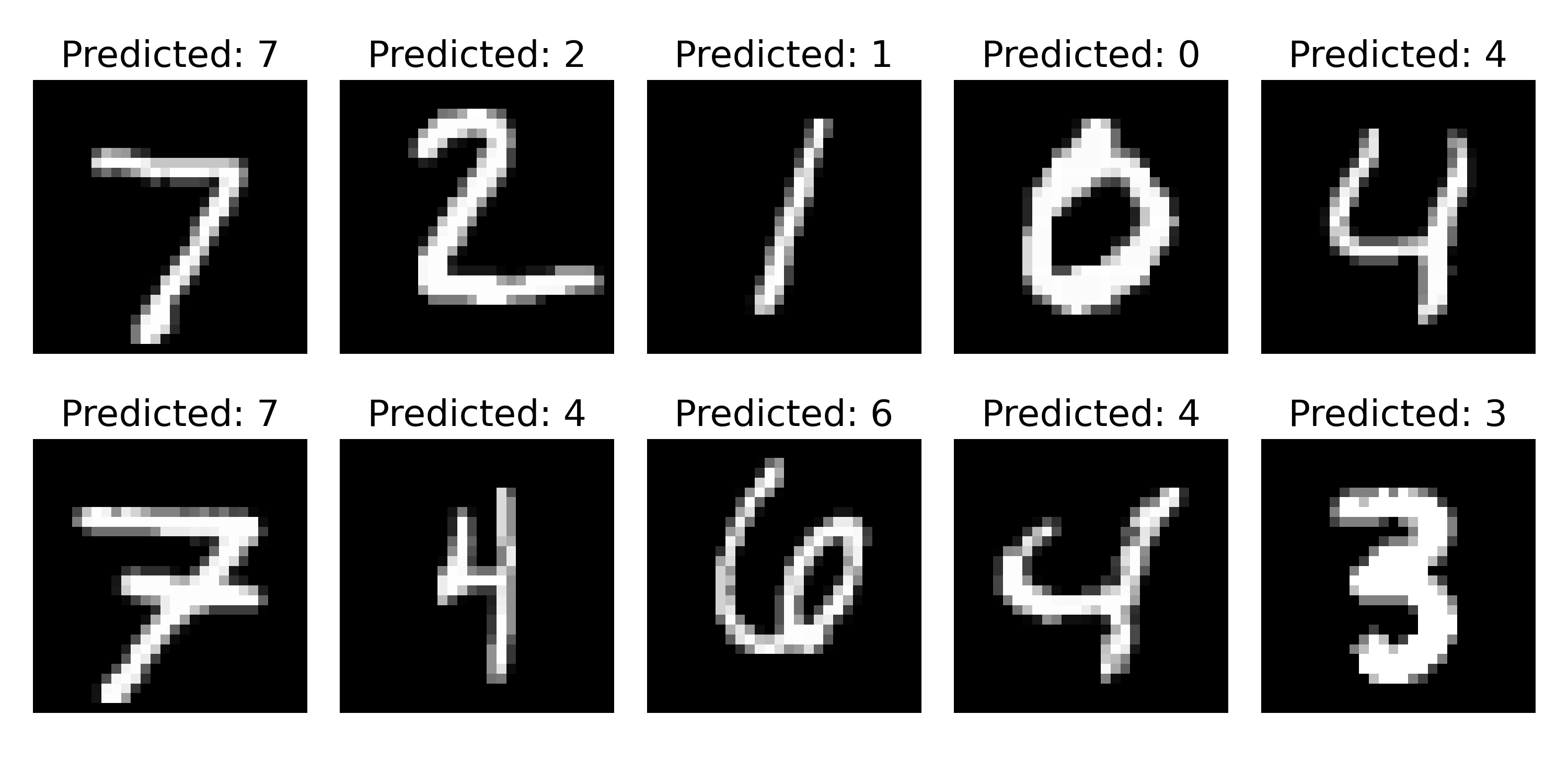Predictions of the CNN on a few test images. The model correctly predicts the labels for most of the images, as shown by the titles below each image. This visual assessment helps understand how the model performs on real data and provides insights into its strengths and weaknesses.

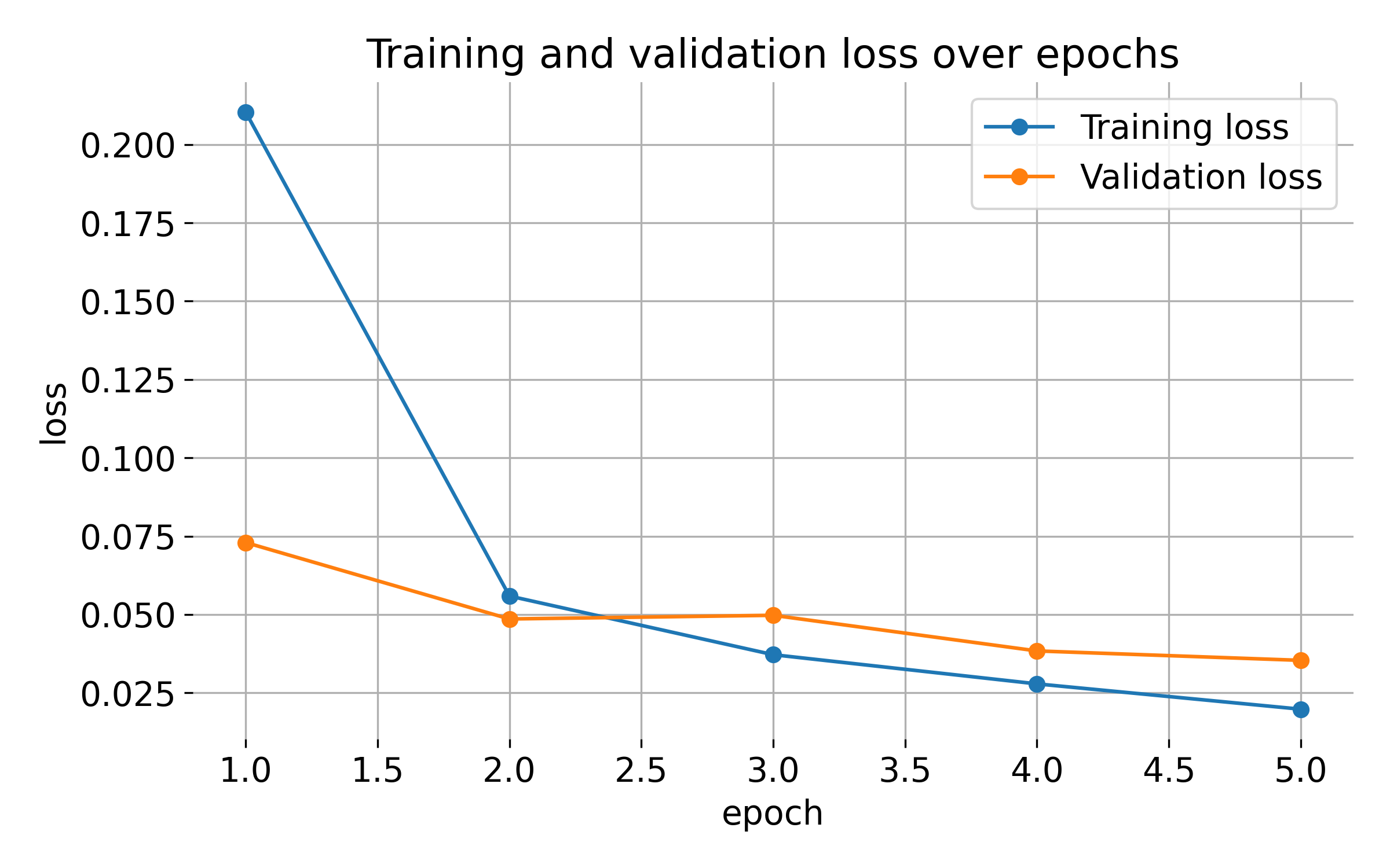Training and validation loss over epochs. The plot shows the training and validation loss decreasing over epochs, indicating that the model is learning from the data and generalizing well. Monitoring the loss helps track the model’s progress and identify potential issues like overfitting or underfitting.

In this example, the model is converging quickly, with the training and validation losses both decreasing sharply in the initial epochs. It also achieves a high accuracy on the test images (98.75%), indicating that the model is performing well on unseen data. However, the loss curves might not look smooth or as “nice” as expected. This can be due to several factors:

• High learning rate: If the learning rate is set too high, the optimizer might take larger steps in the weight space, causing the loss to decrease sharply but not smoothly. Lowering the learning rate could make the loss curves more gradual.
• Small number of epochs: With only 5 epochs, the network is achieving high accuracy very quickly, which might indicate that the model is either relatively simple for the dataset (e.g., MNIST) or overfitting slightly to the training data. Extending training to 10 or 20 epochs could show a more gradual learning curve.
• Batch size: The choice of batch size can also affect the smoothness of loss curves. A smaller batch size often results in noisier gradients and can lead to more fluctuations in the loss.
• Weight initialization: Random initialization can cause some fluctuation in early epochs. Re-initializing the model weights in different ways can sometimes lead to smoother curves, especially in small datasets.
• Regularization: If overfitting is a concern, we might add dropout layers or other regularization techniques, which would also impact the loss curves and prevent the model from converging too quickly.

Keep in mind, that the model is very simple and the dataset is relatively easy (MNIST), so the high accuracy and fast convergence are expected, while improvements can still be made to the model architecture and training process. For more complex datasets or models, the loss curves might look different, and the training process could require more tuning and monitoring to achieve optimal performance.