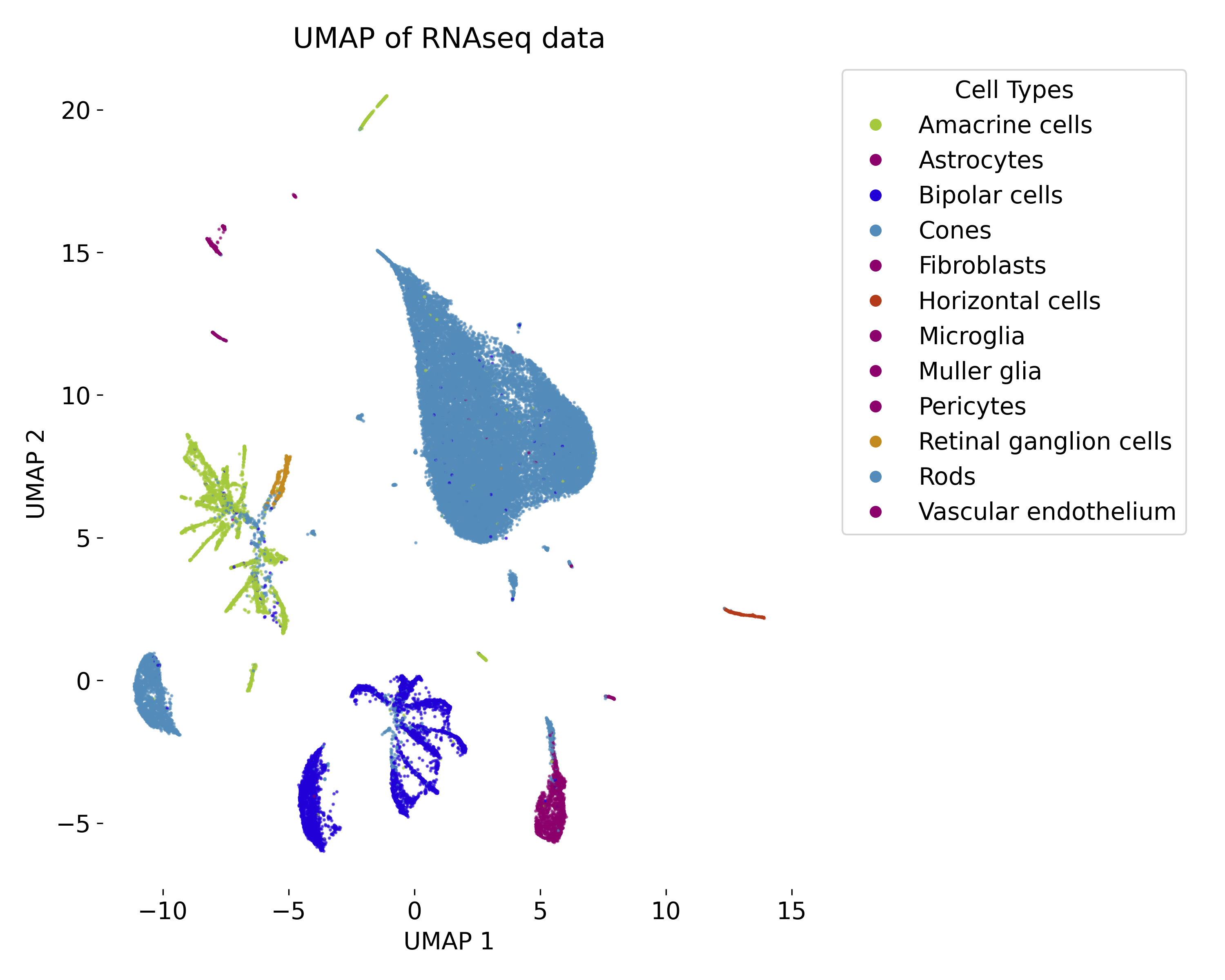
Uniform Manifold Approximation and Projection (UMAP)
UMAP (Uniform Manifold Approximation and Projection) is a non-linear dimensionality reduction method specifically designed for the visualization and exploration of high-dimensional data in lower-dimensional spaces, typically 2D or 3D. Like t-SNE, UMAP excels at preserving local structures, but it also attempts to retain the global structure, making it more suitable for capturing relationships between distant clusters. UMAP is based on the assumption that data lies on a low-dimensional manifold embedded within a higher-dimensional space, and it seeks to map this manifold into a lower-dimensional space while preserving the important structures of the original data.
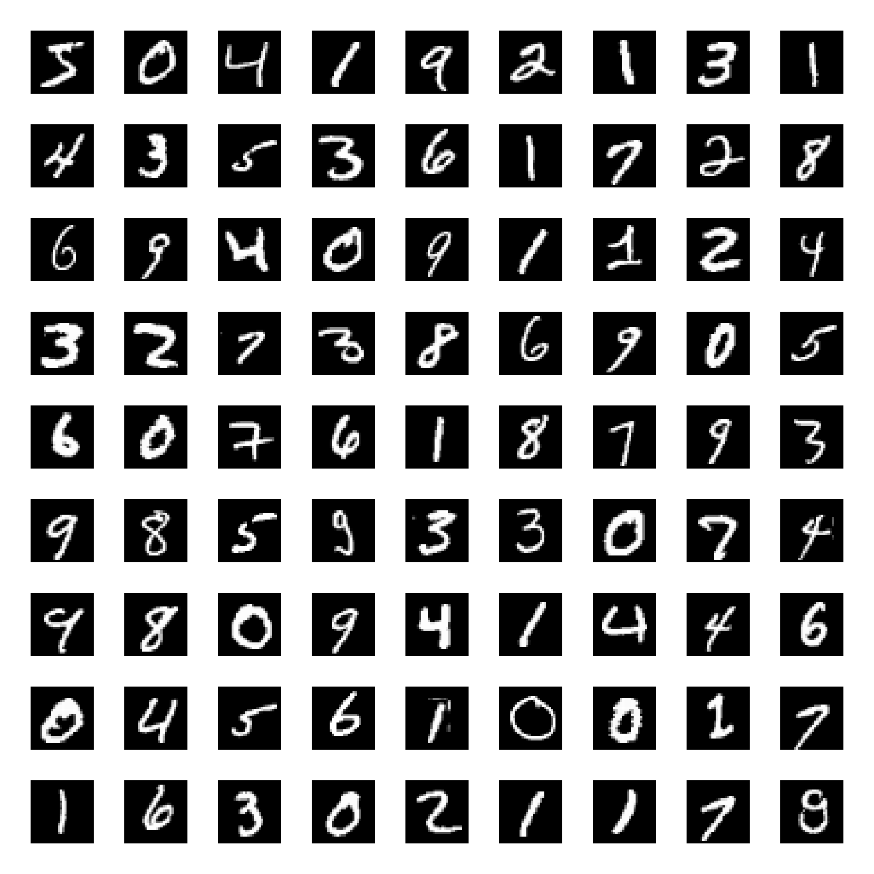
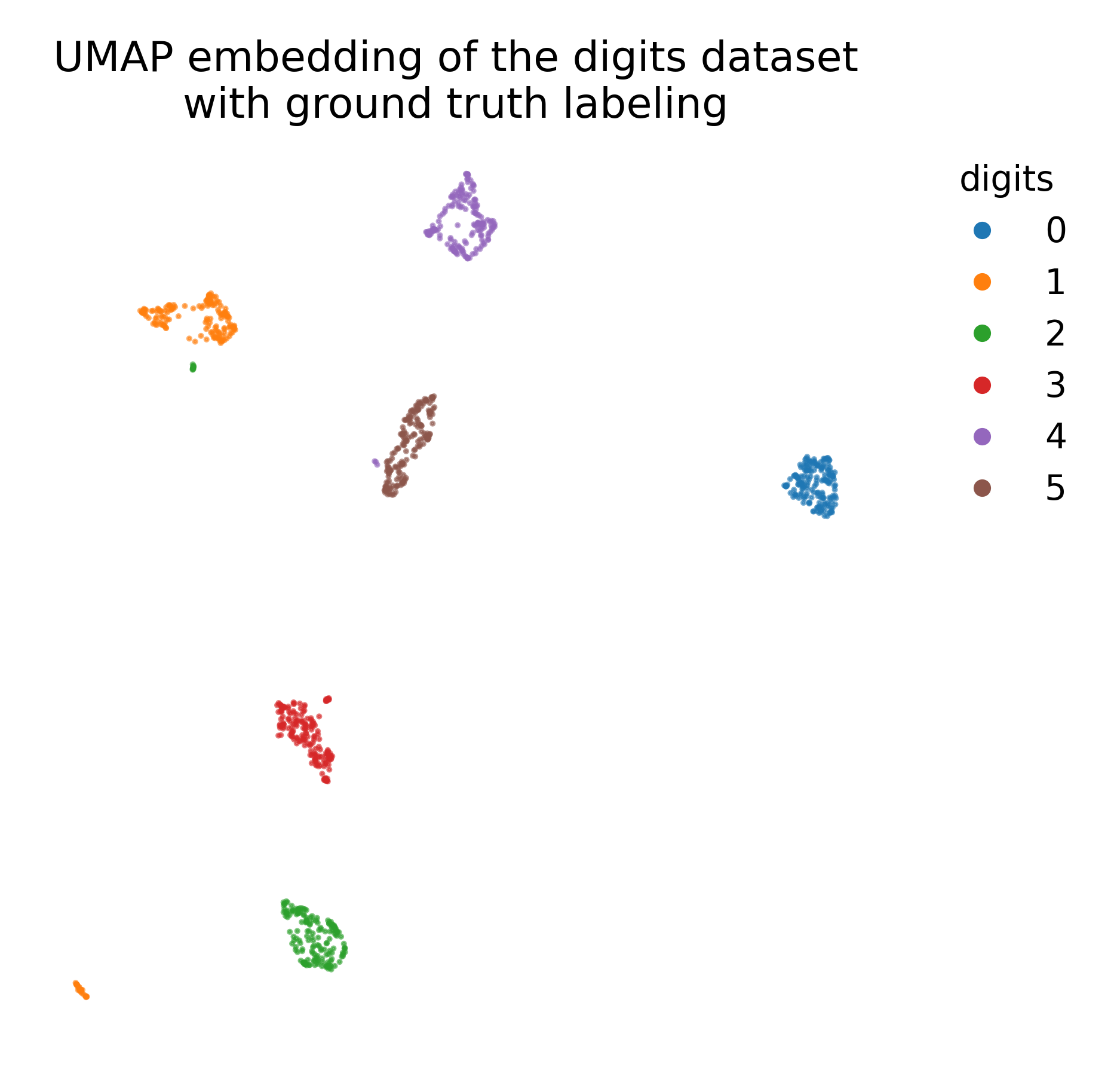
UMAP embedding (right) of the digits dataset (left).
Key concepts in UMAP
Manifold learning
UMAP assumes that the data lies on a low-dimensional manifold, a smooth surface embedded in a higher-dimensional space. The algorithm seeks to learn this underlying manifold structure and represent it accurately in a lower-dimensional space by focusing on local neighborhoods.
Local vs. global structure
- Local structure: UMAP ensures that data points that are close together in the high-dimensional space remain close together in the low-dimensional embedding.
- Global structure: UMAP also attempts to preserve the broader relationships between clusters of points, making it better at maintaining global structure compared to other techniques like t-SNE.
Topology and simplicial complexes
UMAP uses concepts from topology, specifically simplicial complexes, to represent the high-dimensional data as a graph. The simplicial complex helps UMAP model the relationships between points and approximate the underlying manifold.
Algorithm overview
1. Graph construction:
UMAP starts by constructing a weighted k-nearest neighbor (k-NN) graph to capture local relationships in the high-dimensional space. For each point $x_i$, it finds its k-nearest neighbors and assigns weights to the edges of the graph using a Gaussian kernel:
\[p_{ij} = \exp\left( -\frac{||x_i - x_j|| - \rho_i}{\sigma_i} \right)\]where $\rho_i$ is the distance to the nearest neighbor, and $\sigma_i$ is a normalization term controlling the width of the kernel. The graph represents how strongly each point is connected to its neighbors.
2. Fuzzy simplicial complex construction:
Once the k-NN graph is constructed, UMAP builds a fuzzy topological structure, or fuzzy simplicial complex, from the graph. The fuzzy set represents the local connectivity between points as membership strengths, capturing the likelihood that two points are neighbors in the original high-dimensional space.
3. Low-dimensional representation:
In the lower-dimensional space, UMAP models the similarity between two points $y_i$ and $y_j$ using an exponential decay function:
\[q_{ij} = \frac{1}{1 + ||y_i - y_j||^2}\]This function encourages UMAP to maintain the relative distances between points in the low-dimensional embedding, ensuring that points that were close in high dimensions remain close after the reduction.
4. Optimization through cross-entropy loss:
The goal of UMAP is to minimize the difference between the fuzzy simplicial complex in the high-dimensional space and the low-dimensional embedding. This is done by minimizing a cross-entropy loss:
\[\mathcal{L} = - \sum_{i \neq j} \left( p_{ij} \log q_{ij} + (1 - p_{ij}) \log(1 - q_{ij}) \right)\]The loss function penalizes mismatches between the high-dimensional and low-dimensional neighborhoods, ensuring that UMAP preserves the local and global structure during dimensionality reduction. The optimization is performed using stochastic gradient descent to iteratively adjust the positions of the points in the lower-dimensional space.
UMAP Parameters
n_neighbors
This parameter controls the size of the local neighborhood UMAP considers when approximating the manifold structure. Smaller values of n_neighbors focus more on capturing fine, local structures, while larger values capture more global relationships.
- Typical values range from 5 to 50.
min_dist
min_dist controls how tightly UMAP packs points in the low-dimensional space. A smaller min_dist results in more compact clusters, while a larger value leads to a more spread-out embedding.
- Values range from 0.001 to 0.5.
Metric
UMAP supports various distance metrics (e.g., Euclidean, cosine) to compute distances between points in the high-dimensional space. The choice of metric depends on the nature of the data and the type of relationships one wants to preserve.
Advantages and limitations of UMAP
Advantages:
-
Preserves local and global structure: Unlike t-SNE, which excels at preserving local structure but may distort global relationships, UMAP is better at maintaining both local neighborhood relationships and the global layout of the data.
-
Scalability: UMAP is computationally efficient and can handle large datasets, making it suitable for real-world applications that involve high-dimensional data.
-
Flexibility: UMAP supports a wide range of distance metrics, allowing it to be applied to diverse types of data, such as images, text embeddings, or biological data.
-
Stable embeddings: UMAP generally produces more stable embeddings compared to t-SNE, meaning that running the algorithm multiple times with different random seeds tends to result in similar outcomes.
Limitations:
-
Parameter sensitivity: The quality of UMAP’s embeddings can be highly sensitive to the choice of
n_neighborsandmin_dist. These parameters often need to be carefully tuned for different datasets. -
Global structure: Although UMAP does a better job than t-SNE at preserving global structure, it may still distort relationships between clusters in very high-dimensional data.
-
Interpretability: Like other dimensionality reduction techniques, the axes in UMAP’s low-dimensional embedding are not directly interpretable, meaning that the resulting lower-dimensional coordinates do not necessarily correspond to meaningful features in the original data.
Practical considerations
- Preprocessing: It’s important to standardize or normalize the data before applying UMAP to ensure that different features are comparable in scale. Without this step, UMAP may produce misleading results.
- Initial dimensionality reduction: For very high-dimensional datasets, it is common to apply a linear dimensionality reduction technique like PCA first, reducing the dimensionality to a manageable number (e.g., 50), before applying UMAP. This helps UMAP focus on the most important variance in the data.
- Parameter tuning: UMAP requires careful tuning of its
n_neighborsandmin_distparameters depending on the structure of the data. Running UMAP multiple times with different parameter settings can help identify the most meaningful embedding for a particular dataset.
Conclusion
UMAP is a powerful tool for non-linear dimensionality reduction, offering significant advantages in terms of both local and global structure preservation, computational efficiency, and flexibility. Its ability to scale well with large datasets and provide more stable embeddings makes it a popular choice for visualizing and exploring complex high-dimensional data.
UMAP is commonly used in fields such as bioinformatics (e.g., single-cell RNA sequencing), image analysis, and machine learning, where understanding the structure of high-dimensional data is critical for further analysis or interpretation.
Python example
 Samples from the MNIST dataset.
Let’s start by loading the dataset. We will load the digits dataset and only use six first of the ten available classes:
import os
import numpy as np
import matplotlib.pyplot as plt
from sklearn.datasets import load_digits
from sklearn.preprocessing import MinMaxScaler
from sklearn.cluster import KMeans
from sklearn.decomposition import PCA
import umap

digits = load_digits(n_class=6)
X, y = digits.data, digits.target
n_samples, n_features = X.shape
n_neighbors = 30
We use the MinMaxScaler to standardize the data before applying UMAP:
# standardize the data:
X = MinMaxScaler().fit_transform(X)
Next, we apply UMAP to the standardized data:
# UMAP embedding of the digits dataset
umap_model = umap.UMAP(n_neighbors=n_neighbors, n_components=2, random_state=0)
X_umap = umap_model.fit_transform(X)
To visualize the results, we plot the UMAP embedding with and without ground truth color coding:
DIGIT_COLORS = {
    "0": "#1f77b4",
    "1": "#ff7f0e",
    "2": "#2ca02c",
    "3": "#d62728",
    "4": "#9467bd",
    "5": "#8c564b"
    }

# plot the UMAP embedding w/o ground truth color coding:
plt.figure(figsize=(5.15, 6))
plt.scatter(X_umap[:, 0], X_umap[:, 1], c="k", cmap=plt.cm.tab10, alpha=0.5)
plt.title("UMAP embedding of the digits dataset\nwithout ground truth labeling")
plt.xticks([])
plt.yticks([])
plt.show()

# plot the UMAP embedding with ground truth color coding:
plt.figure(figsize=(6.25, 6))
colors = plt.cm.tab10(y)
plt.scatter(X_umap[:, 0], X_umap[:, 1], c=colors, cmap=plt.cm.tab10)
plt.title("UMAP embedding of the digits dataset\nwith ground truth labeling")
plt.xticks([])
plt.yticks([])
# add a 'colorbar' that matches the cell types:
handles = [plt.Line2D([0], [0], marker='o', color='w', markerfacecolor=color, markersize=8, label=label)
           for label, color in DIGIT_COLORS.items()]
plt.legend(handles=handles, title="digits", bbox_to_anchor=(1.05, 1), loc='upper left', frameon=False)
plt.show()
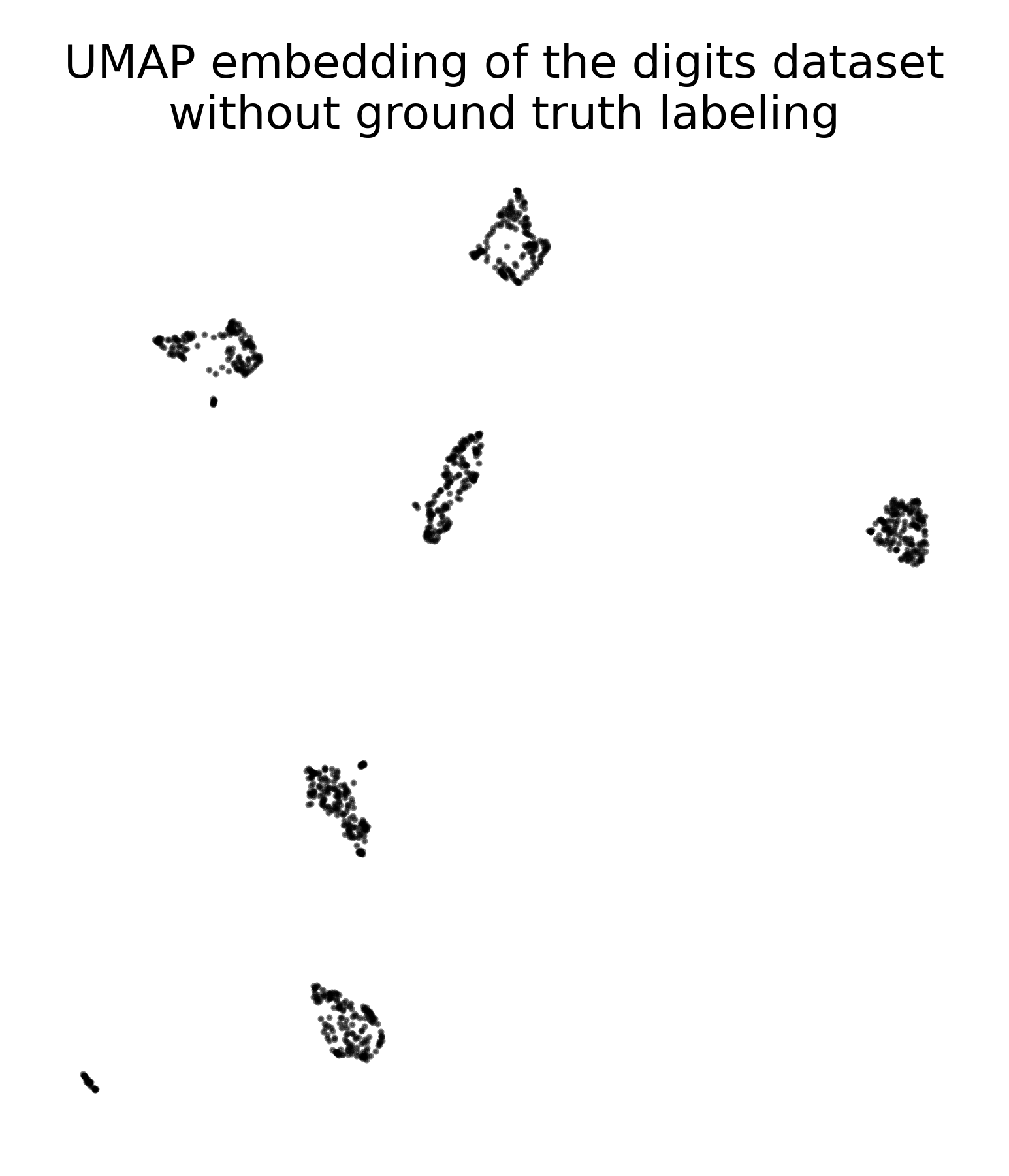 UMAP embedding of the digits dataset without ground truth labeling.
 UMAP embedding of the digits dataset with ground truth labeling.
We can also apply k-means clustering to the UMAP embedding to explore potential clusters in the low-dimensional space (e.g., in case no ground truth labels are available):
# apply k-means clustering to the UMAP embedding:
kmeans = KMeans(n_clusters=6, random_state=0)
kmeans_labels = kmeans.fit_predict(X_umap)

# plot the UMAP embedding with k-means cluster labels:
plt.figure(figsize=(7, 6))
plt.scatter(X_umap[:, 0], X_umap[:, 1], c=kmeans_labels, cmap=plt.cm.tab10)
plt.title("UMAP embedding of the digits dataset\nwith KMeans clustering")
plt.xticks([])
plt.yticks([])
# add a 'colorbar' that matches the cell types:
# create a dictionary to assign the cluster labels the tab10 colors:
cluster_to_color = {i: plt.cm.tab10(i) for i in range(6)}
handles = [plt.Line2D([0], [0], marker='o', color='w', markerfacecolor=plt.cm.tab10(i), markersize=8,
                      label=f"Cluster {i}")
           for i in range(6)]
plt.legend(handles=handles, title="Cluster", bbox_to_anchor=(1.05, 1), loc='upper left', frameon=False)
plt.show()
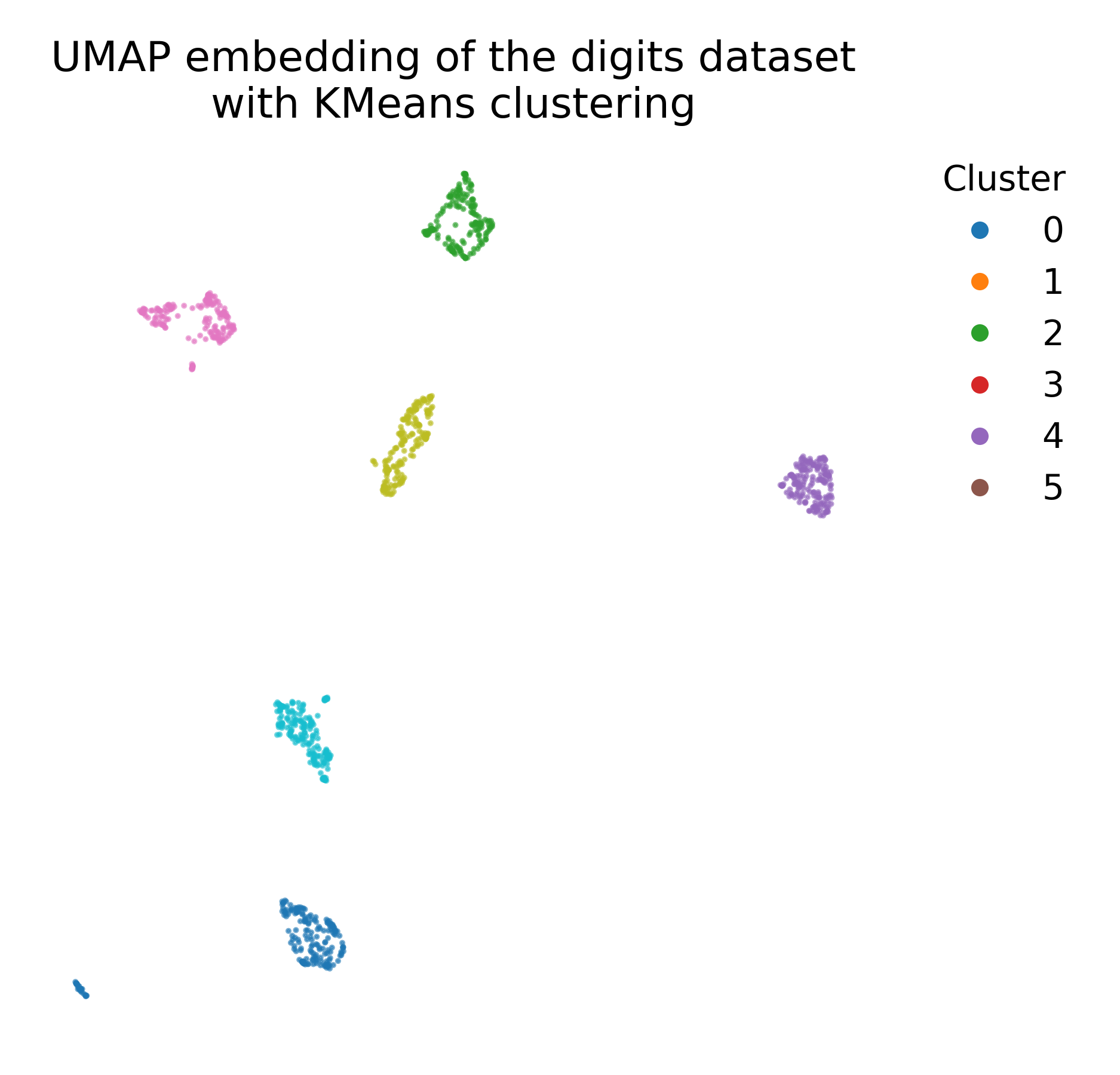

k-means clustering applied to the UMAP embedding of the digits dataset (left), compared to the ground truth labeling (right).
For comparison, we again apply PCA to the data to demonstrate the differences between UMAP and PCA:
pca = PCA(n_components=2)
X_pca = pca.fit_transform(X)

# plot the PCA embedding with ground truth color coding:
plt.figure(figsize=(6, 6))
colors = plt.cm.tab10(y)
plt.scatter(X_pca[:, 0], X_pca[:, 1], c=colors, cmap=plt.cm.tab10)
plt.title("PCA embedding of the digits dataset\nwith ground truth labeling")
plt.xticks([])
plt.yticks([])
# add a 'colorbar' that matches the cell types:
handles = [plt.Line2D([0], [0], marker='o', color='w', markerfacecolor=color, markersize=8, label=label)
           for label, color in DIGIT_COLORS.items()]
plt.legend(handles=handles, title="digits", bbox_to_anchor=(1.05, 1), loc='upper left', frameon=False)
plt.show()
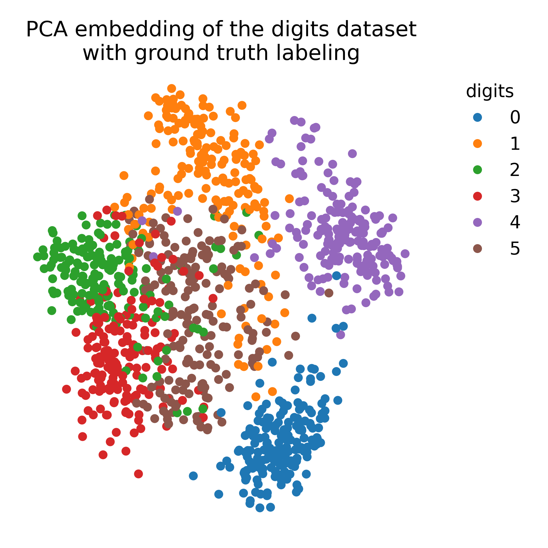 PCA embedding of the digits dataset with ground truth labeling.
Exercise
In the exercise, we will apply UMAP to a RNAseq dataset and explore the resulting low-dimensional embedding. We will compare the UMAP visualization with the ground truth labels and vary the parameters of the model to observe the impact on the embedding.
