Clustering methods

Clustering is a type of unsupervised machine learning technique that is used to group data points into distinct clusters based on similarity. Unlike supervised learning, clustering does not require labeled data. The primary goal is to group data points in such a way that points in the same group (cluster) are more similar to each other than to those in other groups. Clustering techniques have broad applications in fields such as data analysis, image processing, and bioinformatics. With regard to dimensionality reduction, clustering can be used to identify patterns in the reduced feature space and to group similar data points together. In this chapter, we will discuss three common clustering methods: k-Means, agglomerative clustering, and DBSCAN, highlighting their objectives, algorithms, strengths, and limitations.

Different clustering methods can be used to group data points into distinct clusters based on similarity. Each method has its own strengths and limitations, making it suitable for different types of data and applications.

k-Means clustering

k-Means is a popular partitional clustering algorithm that aims to divide $n$ data points into $k$ distinct clusters. Each data point is assigned to the cluster whose centroid (the mean of the points in the cluster) is closest, based on a distance metric (typically Euclidean distance).

The primary goal of k-Means is to minimize the within-cluster variance (also called inertia) by iteratively assigning data points to clusters and updating the centroids until convergence.

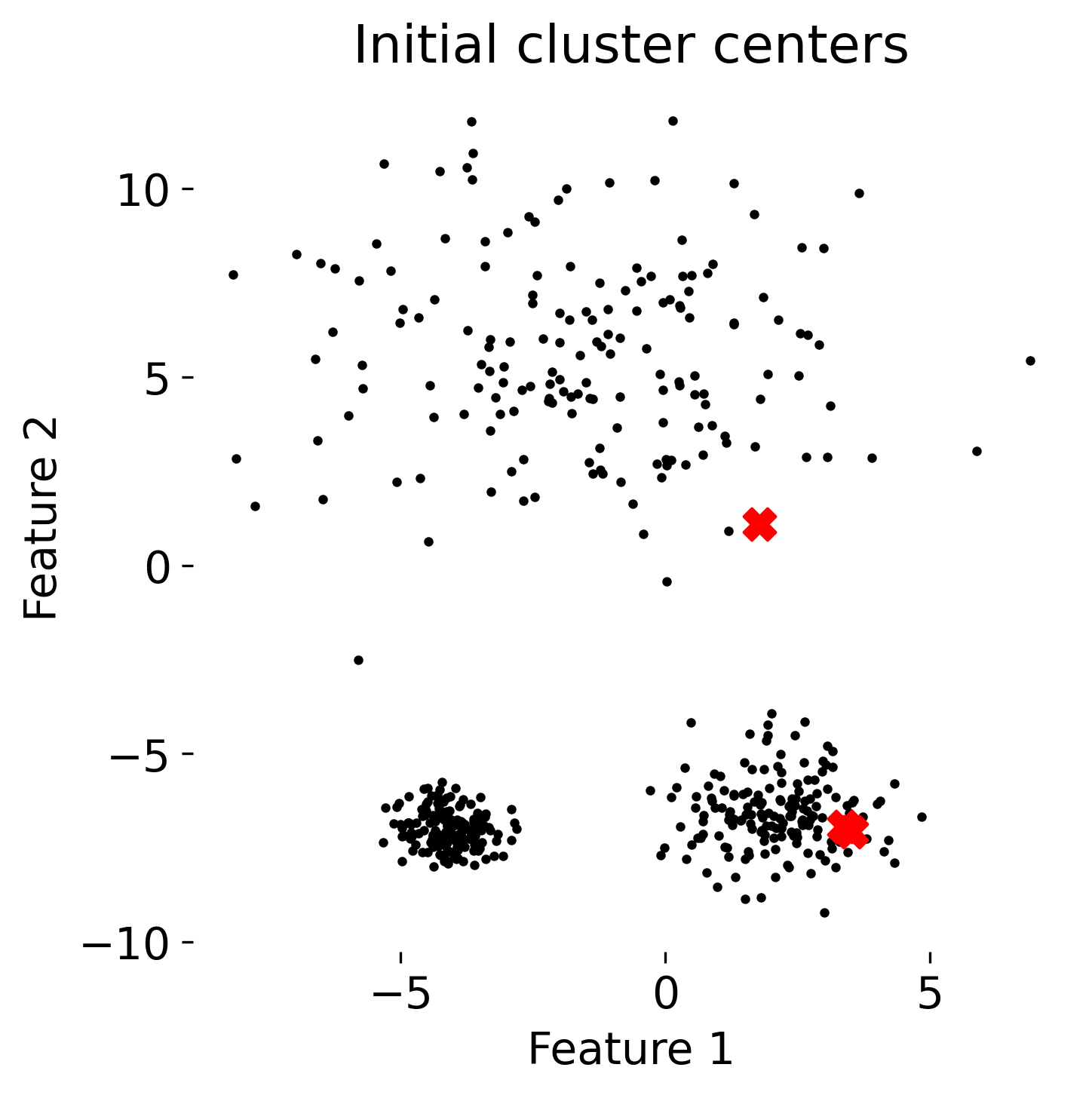
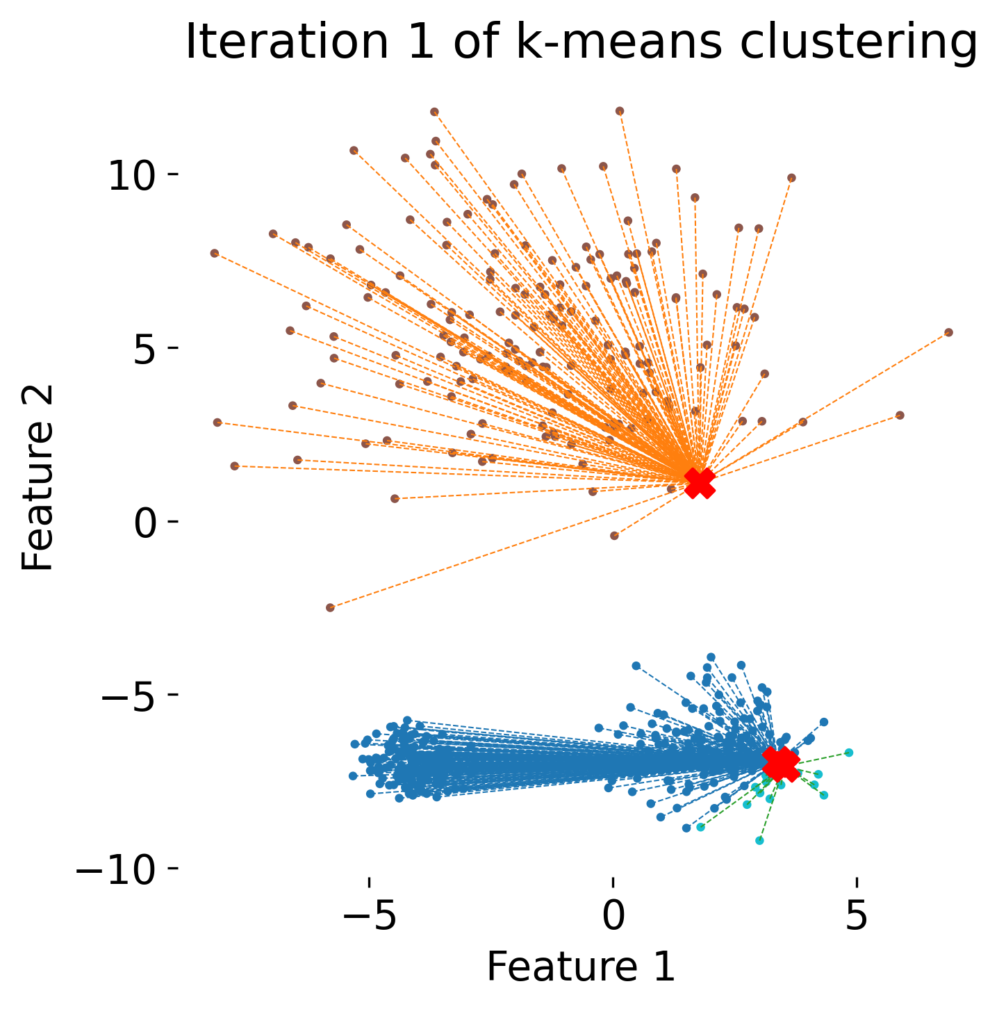
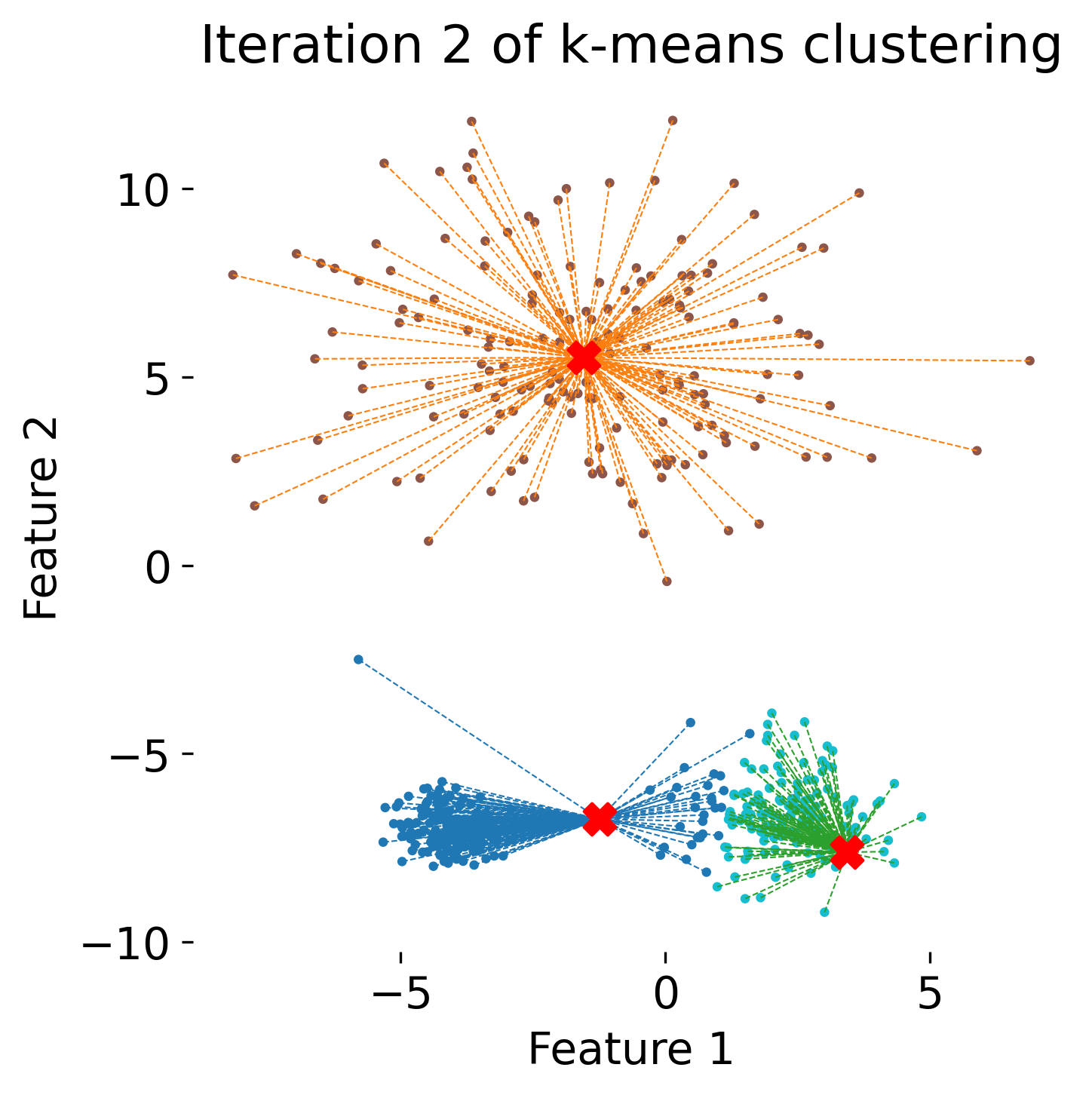
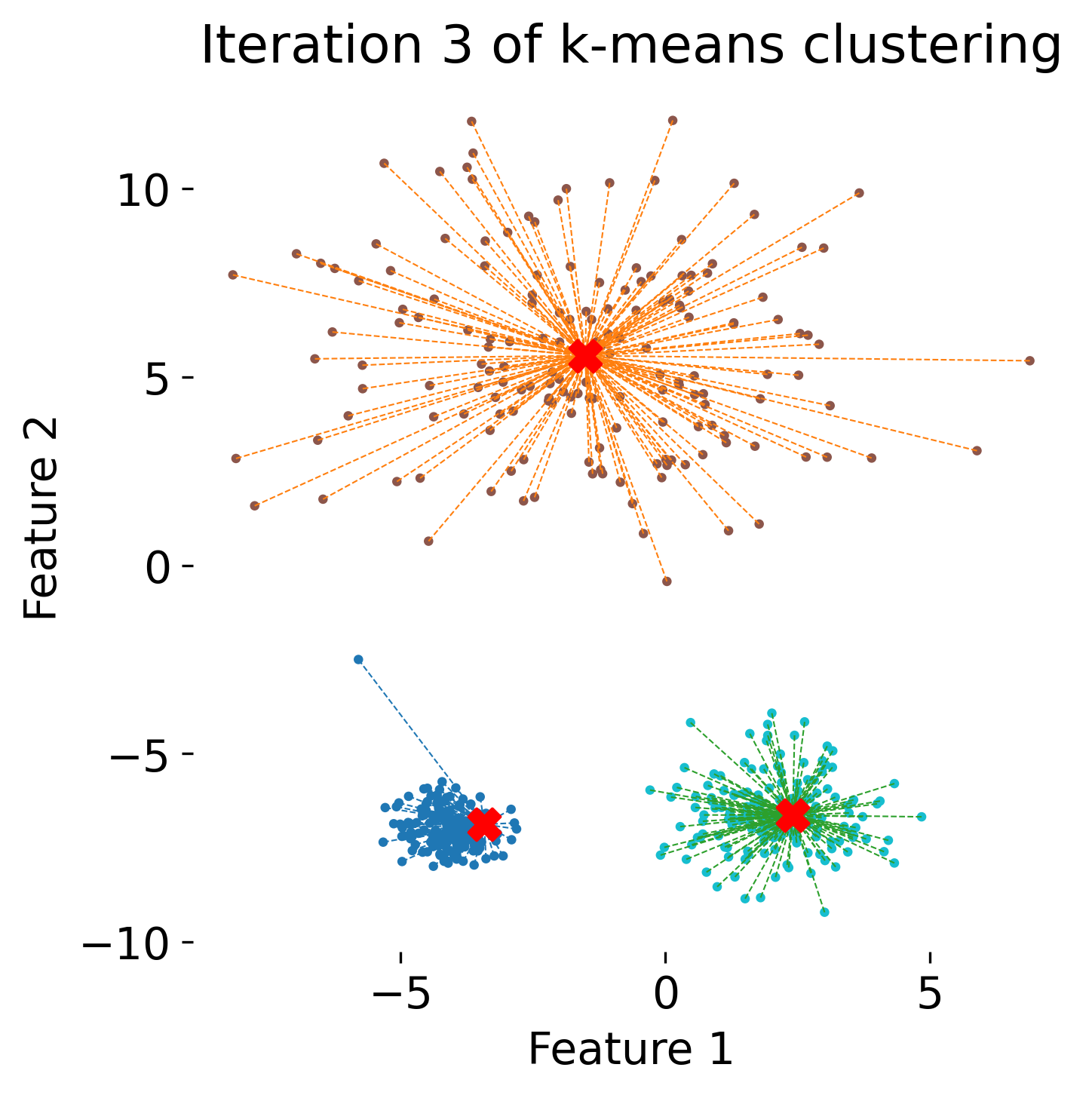
The figure illustrates the process of k-means clustering applied to a toy dataset with three clusters. The first panel shows the initial random placement of centroids (red ‘X’ markers). In the subsequent four panels, the algorithm iteratively updates the cluster centers. Each iteration consists of two steps: 1) assigning each data point (represented by colored dots) to the nearest centroid based on Euclidean distance, indicated by dashed gray lines, and 2) recalculating the centroids as the mean position of the data points in each cluster. Over the iterations, the centroids converge to their final positions, minimizing the within-cluster distances and leading to stable cluster assignments.

Algorithm overview

1. Initialization

Select $k$ random points as initial centroids.

2. Assignment step

Assign each data point to the nearest centroid based on the distance metric. Each point $x_i$ is assigned to the cluster $C_j$ with the nearest centroid:

\[C_j = \{ x_i : \arg \min_j ||x_i - \mu_j||^2 \}\]

Update step

Recompute the centroids of the clusters by taking the mean of the points in each cluster:

\[\mu_j = \frac{1}{|C_j|} \sum_{x_i \in C_j} x_i\]

4. Repeat

Iterate between the assignment and update steps until convergence (i.e., no further changes in assignments or centroids).

Objective function

The objective of k-Means is to minimize the within-cluster sum of squared distances (WCSS), often referred to as inertia:

\[\text{WCSS} = \sum_{j=1}^{k} \sum_{x_i \in C_j} ||x_i - \mu_j||^2\]

This function measures the compactness of clusters, and the algorithm seeks to minimize this value.

Silhouette score and plot

The silhouette score is a metric used to evaluate the quality of clustering results. It measures how similar an object is to its own cluster compared to other clusters. The silhouette score ranges from -1 to 1, where a higher score indicates better clustering. A score close to 1 indicates that the data points are well-clustered, while a score close to -1 suggests that the data points may be assigned to the wrong clusters.

Example silhouette plot for k-Means clustering with anisotropic data. The plot shows the silhouette scores for each data point, with the average silhouette score indicated by a vertical line. A higher average silhouette score indicates better clustering results.

The silhouette score is calculated as follows:

\[s_i = \frac{b_i - a_i}{\max(a_i, b_i)}\]

where $a_i$ is the average distance between point $i$ and all other points in the same cluster, and $b_i$ is the average distance between point $i$ and all points in the nearest cluster (other than its own).

By averaging the silhouette scores of all data points, we obtain the overall average silhouette score for the clustering result.

A silhouette plot can be generated to visualize the silhouette scores for each data point. The plot shows the silhouette score for each point as well as the average silhouette score for the entire dataset. A higher average silhouette score indicates better clustering results, while negative scores within a cluster suggest that the clustering may be suboptimal.

Convergence and complexity

k-Means converges when the assignments of points to clusters do not change between iterations or when centroids stabilize. However, it only guarantees convergence to a local minimum and may not find the global optimum.

The complexity of each iteration of k-Means is $O(n \cdot k \cdot d)$, where $n$ is the number of data points, $k$ is the number of clusters, and $d$ is the dimensionality of the data.

Strengths and limitations

Strengths:

• Simple to implement and efficient on large datasets
• Works well when clusters are roughly spherical and have equal sizes

Limitations:

• Requires predefining the number of clusters $k$
• Sensitive to the initial placement of centroids
• Not effective for non-spherical or unevenly sized clusters
• Sensitive to outliers and noise

Python example

We will first generate some example data sets, that cover different types of distributions and data structures:

import os
import numpy as np
import pandas as pd
import matplotlib.pyplot as plt
import matplotlib.cm as cm

from sklearn import cluster, datasets
from sklearn.preprocessing import StandardScaler

from scipy.cluster.hierarchy import dendrogram
from scipy.cluster.hierarchy import linkage
from scipy.spatial.distance import pdist
from sklearn.metrics import silhouette_samples, silhouette_score

# for reproducibility, we set the seed:
np.random.seed(0)

# generate some test data:
# noisy_circles and noisy_moons:
n_samples = 500
seed = 30
noisy_circles = datasets.make_circles(n_samples=n_samples, factor=0.5, noise=0.05, random_state=seed)
noisy_moons = datasets.make_moons(n_samples=n_samples, noise=0.05, random_state=seed)
blobs = datasets.make_blobs(n_samples=n_samples, random_state=seed)
rng = np.random.RandomState(seed)
no_structure = rng.rand(n_samples, 2), None

# anisotropicly distributed data with different variances:
random_state = 170
X, y = datasets.make_blobs(n_samples=n_samples, random_state=random_state)
transformation = [[0.6, -0.6], [-0.4, 0.8]]
X_aniso = np.dot(X, transformation)
aniso = (X_aniso, y)

# blobs with varied variances:
varied = datasets.make_blobs(n_samples=n_samples, cluster_std=[1.0, 2.5, 0.5], random_state=random_state)

# plot all datasets:
datasets_all = [noisy_circles, noisy_moons, varied, aniso, blobs, no_structure]
dataset_names = ['Noisy circles', 'Noisy moons', 'Varied variances', 'Anisotropic', 'Blobs', 'No structure']
fig, ax = plt.subplots(1, 6, figsize=(20, 4))
# iterate over datasets:
for idx, dataset in enumerate(datasets_all):
    X, y = dataset
    # standardize the data:
    X = StandardScaler().fit_transform(X)
    ax[idx].scatter(X[:, 0], X[:, 1], s=10)
    ax[idx].set_xticks([])
    ax[idx].set_yticks([])
    ax[idx].set_title(f'{dataset_names[idx]}')
# add a main title:
plt.suptitle('Different, unclustered datasets')
plt.show()

Six example datasets with varying structures and distributions. These datasets will be used to demonstrate clustering methods.

Next, we demonstrate how to cluster these datasets using k-Means clustering from scikit-learn. We exemplarily show how to cluster one of the datasets generated above (e.g., “blobs”):

blobs_data = datasets_all[4] # select the "blobs" dataset

# define the number of clusters:
n_clusters = 3

# create the KMeans object:
kmeans = cluster.KMeans(n_clusters=n_clusters, random_state=0)

# fit the data:
kmeans_fit = kmeans.fit(blobs_data[0])

kmeans_fit is the fitted k-Means model. It contains (among other useful information) the cluster assignments in kmeans_fit.labels_ and the cluster centers in kmeans_fit.cluster_centers_.

With the determined cluster assignments, we can then plot the clustering results by color-coding the data points by the cluster labels (kmeans_fit.labels_):

# plot the clustering results:
fig, ax = plt.subplots(1, 1, figsize=(6, 6))
ax.scatter(blobs_data[0][:, 0], blobs_data[0][:, 1], c=kmeans_fit.labels_, s=10)
# indicate the cluster centers:
ax.scatter(kmeans_fit.cluster_centers_[:, 0], kmeans_fit.cluster_centers_[:, 1], c='r', s=100, marker='x')
ax.set_title(f'KMeans clustering ({n_clusters} clusters)')
plt.show()

k-means clustering results (right) for three clusters of the blobs dataset (left). Cluster centers are marked with red crosses.

Let’s investigate the cluster assignments and the centroids:

print(f"shape of the data:   {blobs_data[0].shape}")
print(f"shape of the labels: {kmeans_fit.labels_.shape}")

shape of the data:   (500, 2)
shape of the labels: (500,)

print(f"KMeans labels: {kmeans_fit.labels_}")

KMeans labels: [0 1 1 0 2 0 2 0 1 2 1 1 1 2 0 2 1 1 1 2 0 2 1 2 1 0 0 0 1 1 1 0 0 0 2 2 0
 1 0 1 1 2 2 2 1 2 1 2 1 1 1 2 1 1 2 2 0 2 2 1 2 1 2 0 0 0 1 2 0 2 2 0 2 1
 1 1 0 2 0 2 1 2 0 0 1 0 1 0 1 0 2 0 1 2 1 1 1 0 1 0 2 2 1 1 2 2 1 1 2 1 1
 2 0 1 2 1 0 0 2 0 0 2 2 2 0 0 0 1 1 2 2 1 2 1 2 0 0 2 1 0 1 1 0 2 2 0 1 1
 2 2 1 0 1 0 2 0 0 0 1 1 2 1 1 2 2 2 1 0 1 1 2 0 0 0 2 0 2 0 0 2 0 2 0 1 2
 0 2 0 0 0 0 0 1 2 2 0 2 0 2 0 2 2 2 0 1 0 2 2 2 0 0 1 2 1 0 0 1 0 2 1 0 2
 1 1 2 0 1 1 0 2 1 1 2 0 1 0 2 2 1 1 2 0 1 0 0 1 1 1 0 0 2 0 2 2 2 0 2 1 1
 1 2 2 2 0 1 1 1 2 2 1 0 1 2 2 0 2 2 2 2 2 0 1 1 2 2 0 1 0 0 2 1 1 1 0 2 2
 0 1 1 1 1 0 1 1 0 1 0 0 1 2 0 1 1 0 1 1 2 0 2 0 1 2 1 1 1 2 1 1 1 0 0 2 0
 0 0 0 2 1 2 0 0 0 2 2 2 0 1 2 2 2 0 2 0 2 0 2 2 2 0 1 2 2 1 0 1 1 1 1 0 1
 1 0 0 0 1 2 2 0 1 2 1 1 1 0 0 1 0 1 0 2 2 0 2 2 0 2 0 1 1 1 0 0 0 1 2 1 2
 0 2 0 2 2 2 1 0 2 0 0 0 0 2 2 1 0 0 2 1 2 0 2 2 1 2 0 1 0 0 1 2 1 0 2 1 1
 1 2 1 0 2 2 0 1 2 2 2 0 2 1 0 1 0 0 0 0 1 1 0 2 0 2 0 2 2 0 1 1 1 1 0 0 2
 1 1 0 0 1 0 0 1 2 0 1 0 0 2 2 0 0 0 1]

print(f"KMeans cluster centers: {kmeans_fit.cluster_centers_}")

KMeans cluster centers: [[ 2.89175588 -2.43710117]
 [ 9.38171445 -2.97689609]
 [ 3.23881011 -6.81817932]]

Here are the results for all datasets:

k-means clustering results for two clusters (upper panel) and three clusters (lower panel) on different datasets.

For calculating the silhouette score and plotting the silhouette plot, we need to define a helper-function that performs these tasks first:

# helper-function to plot the silhouette score:
def plot_silhouette_score(fitted_model, PCA_model_S3_fit, method='kmeans', n_clusters=2):
    # get the cluster labels:
    labels = fitted_model.labels_
    n_clusters = len(np.unique(labels))

    # compute the silhouette scores for each sample:
    silhouette_vals = silhouette_samples(PCA_model_S3_fit, labels)

    # compute the mean silhouette score:
    silhouette_avg = silhouette_score(PCA_model_S3_fit, labels)
    print(f"Mean silhouette score: {silhouette_avg}")
    """ 
    silhouette_score returns the mean Silhouette Coefficient over all samples.
    """

    # create a silhouette plot:
    fig, ax1 = plt.subplots(1, 1)
    fig.set_size_inches(7, 6)

    ax1.set_xlim([-0.1, 1]) # the silhouette coefficient can range from -1, 1
    ax1.set_ylim([0, len(PCA_model_S3_fit) + (n_clusters + 1) * 10])
    # the (n_clusters+1)*10 is for inserting blank space between silhouette plots of individual clusters

    y_lower = 10
    for i in range(n_clusters):
        # aggregate the silhouette scores for samples belonging to cluster i, and sort them:
        ith_cluster_silhouette_vals = silhouette_vals[labels == i]
        ith_cluster_silhouette_vals.sort()

        size_cluster_i = ith_cluster_silhouette_vals.shape[0]
        y_upper = y_lower + size_cluster_i

        color = cm.viridis(float(i) / n_clusters)
        ax1.fill_betweenx(np.arange(y_lower, y_upper),
                        0, ith_cluster_silhouette_vals,
                        facecolor=color, edgecolor=color, alpha=1.0)

        # label the silhouette plots with their cluster numbers at the middle:
        ax1.text(-0.05, y_lower + 0.5 * size_cluster_i, str(i))

        # compute the new y_lower for next plot:
        y_lower = y_upper + 10  # 10 for the 0 samples

    ax1.set_title("The silhouette plot for the various clusters.")
    ax1.set_xlabel("The silhouette coefficient values")
    ax1.set_ylabel("Cluster label")

    # plot a vertical line for the average silhouette score of all the values:
    ax1.axvline(x=silhouette_avg, color="red", linestyle="--")

    ax1.set_yticks([])  # Clear the yaxis labels / ticks
    ax1.set_xticks(np.arange(-0.1, 1.1, 0.2))

    plt.tight_layout()
    plt.savefig(os.path.join(RESULTSPATH, f'{method} silhouette_plot ({n_clusters} clusters).png'), dpi=300)
    plt.show()

Here is an example of how to use this function to plot the silhouette score for the previous k-Means clustering results:

plot_silhouette_score(kmeans_fit, blobs_data[0], method='clustering_kmeans_blobs', n_clusters=n_clusters)

The silhouette plots for the blobs, noisy circles, and anisotropic datasets with two and three clusters are shown below:

Silhouette plots for k-means clustering results with two clusters (upper panel) and three clusters (lower panel) the data sets: blobs, noisy circles, and aniostropic, respectively. Note, that silhouette scores are not always reliable for evaluating clustering results, especially when the clusters are not well-separated. Here, we can see that for both cluster sizes and for the three different datasets, the silhouette scores reveal a good clustering structure. However, the visual inspection of the clustering results shows that the k-means algorithm is not always able to capture the true underlying structure of the data.

Agglomerative clustering

Agglomerative clustering is a type of hierarchical clustering that builds a hierarchy of clusters in a bottom-up manner. Initially, each data point is treated as its own cluster, and clusters are iteratively merged based on proximity until all points are in a single cluster or a stopping criterion is met.

The goal is to create a hierarchy (represented as a dendrogram) that reveals the structure of data at various levels of granularity, offering flexibility in the selection of clusters.

This figure depicts the dendrogram generated by agglomerative hierarchical clustering, a bottom-up clustering method. The algorithm starts by treating each data point as its own individual cluster (bottom level of the dendrogram). In each step, the two clusters that are closest to each other (based on a chosen distance metric) are merged. This process continues iteratively until all points are grouped into a single cluster (top level of the dendrogram). The vertical lines in the dendrogram represent cluster merges, with the height of each line indicating the distance between the clusters being merged. The dendrogram allows for the determination of an optimal number of clusters by cutting the tree at a specific height, which represents the maximum allowable distance between merged clusters.

Algorithm overview

1. Start with individual points: Each data point is treated as a separate cluster.
2. Merge clusters: At each step, merge the two closest clusters based on a distance metric.
3. Repeat: Continue merging clusters until only one cluster remains or the desired number of clusters is achieved.
4. Dendrogram: The merging process is represented as a dendrogram, a tree-like structure that shows how clusters were merged at different distances.

The algorithm steps are thus as follows:

1. Start with individual points

Initially, each data point $x_i$ (where $i = 1, 2, \dots, n$ for $n$ data points) is treated as a singleton cluster:

\[C_i = \{x_i\} \quad \text{for all} \ i \in \{1, 2, \dots, n\}\]

At this stage, there are $n$ clusters.

2. Merge clusters

At each iteration, identify the pair of clusters $C_i$ and $C_j$ that are closest to each other based on a distance metric $d(C_i, C_j)$. The distance between clusters can be defined in various ways depending on the linkage criteria (e.g., single linkage, complete linkage, or average linkage):

• Single Linkage (minimum distance): \(d(C_i, C_j) = \min_{x \in C_i, y \in C_j} ||x - y||\)
• Complete Linkage (maximum distance): \(d(C_i, C_j) = \max_{x \in C_i, y \in C_j} ||x - y||\)
• Average Linkage (average distance): \(d(C_i, C_j) = \frac{1}{|C_i| \cdot |C_j|} \sum_{x \in C_i} \sum_{y \in C_j} ||x - y||\)

Merge the two closest clusters:

\[C_{\text{new}} = C_i \cup C_j\]

After each merge, the total number of clusters decreases by one.

3. Repeat

Continue merging the closest clusters iteratively. After each merge, update the distance matrix to reflect the distance between the newly formed cluster and the remaining clusters.

Formally, the cluster distance matrix $D$ (of size $n \times n$) is updated at each step by recalculating the distances between the merged cluster $C_{\text{new}}$ and all other clusters. This process repeats until only one cluster remains or the desired number of clusters $k$ is reached.

4. Dendrogram

The sequence of merges is represented by a dendrogram, which is a binary tree-like structure. Each branch point (or node) of the dendrogram corresponds to a merge event between two clusters at a certain distance.

The height of a node in the dendrogram reflects the distance between the merged clusters at that stage:

\[h(C_i, C_j) = d(C_i, C_j)\]

By cutting the dendrogram at a specific height (distance threshold), a desired number of clusters can be obtained.

The dendrogram provides a visual representation of the cluster hierarchy. By “cutting” the dendrogram at a specific height (distance), one can select a desired number of clusters. The height of each node represents the distance between the merged clusters.

Computational complexity

Agglomerative clustering has a time complexity of $O(n^3)$ in its naive implementation, making it computationally expensive for large datasets. Optimized algorithms can reduce the complexity to $O(n^2 \log n)$, but it remains costly compared to other methods.

Strengths and Limitations

Strengths:

• Does not require specifying the number of clusters in advance.
• Can handle non-spherical clusters and varying cluster sizes.
• Produces a full hierarchy of clusters for flexible analysis.

Limitations:

• Computationally expensive, especially for large datasets.
• Sensitive to noise and outliers.
• The choice of linkage criteria can greatly affect the resulting clusters.

Python example

Like for k-means, in its simplest form, agglomerative clustering can be performed by executing two lines of Python code:

# define the number of clusters:
n_clusters = 3

# create the Agglomerative object:
agg = cluster.AgglomerativeClustering(n_clusters=n_clusters)

# fit the data:
agg_fit = agg.fit(blobs_data[0])

Check whether the clustering results are as expected (should have the same shape as the data):

print(f"shape of the labels: {agg_fit.labels_.shape}")

shape of the labels: (500,)

And plot the clustering results:

# investigate the results:
print(f"shape of the data: {blobs_data[0].shape}")
print(f"shape of the labels: {agg_fit.labels_.shape}")

print(f"Agglomerative labels: {agg_fit.labels_}")

# plot the clustering results:
fig, ax = plt.subplots(1, 1, figsize=(5, 5))
ax.scatter(blobs_data[0][:, 0], blobs_data[0][:, 1], c=agg_fit.labels_, s=10)
ax.set_title(f'Agglomerative clustering ({n_clusters} clusters)')
plt.show()

Agglomerative clustering results (right) for three clusters of the blobs dataset (left).

Here is the plot for all datasets:

Agglomerative clustering results for two clusters (upper panel) and three clusters (lower panel) on all datasets.

In order gain a deeper insight into the hierarchical structure of the clusters, we can also plot the dendrogram for the blobs dataset:

# we need to calculate the linkage matrix first:
agg = cluster.AgglomerativeClustering(n_clusters=n_clusters)
agg.fit(blob_data)

# calculate the linkage matrix:
Z = linkage(X, 'ward')

# finally, plot the dendrogram:
fig, ax = plt.subplots(1, 1, figsize=(10, 5))
dendrogram(Z, ax=ax)
plt.title('Dendrogram')
plt.savefig(RESULTSPATH + f'clustering_agg_dendrogram_blobs_dataset.png', dpi=300)
plt.show()

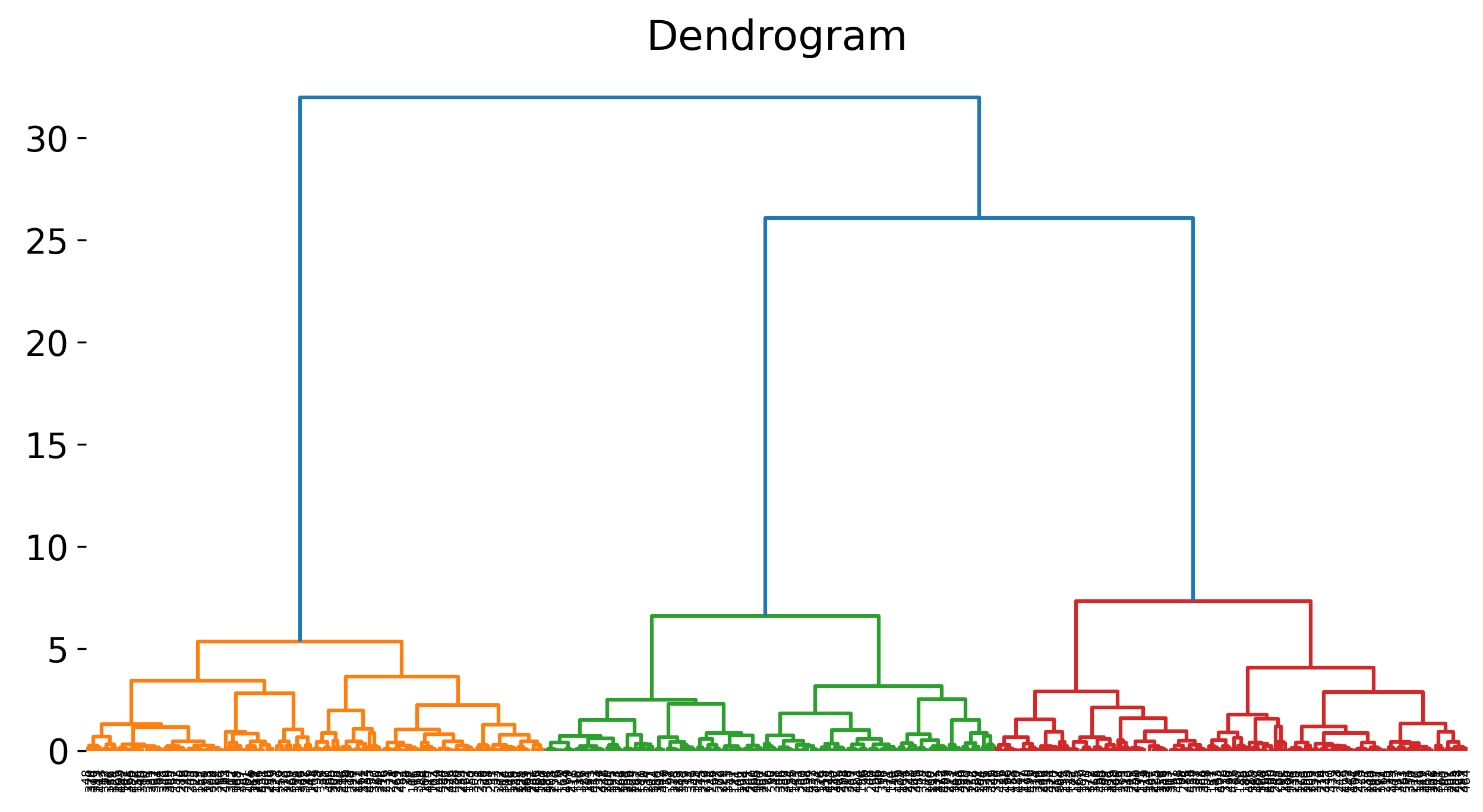Dendrogram for the blobs dataset, showing the hierarchical structure of the clusters.

The according silhouette plots for three example datasets are shown below:

Silhouette plots for agglomerative clustering results with two clusters (upper panel) and three clusters (lower panel) the data sets: blobs, noisy circles, and aniostropic, respectively.

DBSCAN (Density-Based Spatial Clustering of Applications with Noise)

DBSCAN (Density-Based Spatial Clustering of Applications with Noise) is a density-based clustering algorithm that groups points in dense regions while identifying points in low-density regions as noise. Unlike k-Means or hierarchical clustering, DBSCAN does not require specifying the number of clusters in advance and can form clusters of arbitrary shapes.

Key concepts in DBSCAN

Core points

A point $x_i$ is classified as a core point if it has at least $\text{MinPts}$ neighbors within a radius $\epsilon$, meaning:

\[|N_{\epsilon}(x_i)| \geq \text{MinPts}\]

where $N_{\epsilon}(x_i) = {x_j \in X : d(x_i, x_j) \leq \epsilon }$ is the set of points within the $\epsilon$-neighborhood of $x_i$, and $d(x_i, x_j)$ is typically the Euclidean distance between points $x_i$ and $x_j$.

Border points

A point $x_i$ is a border point if it is not a core point but lies within the $\epsilon$-neighborhood of a core point. Formally, $x_i$ is a border point if:

\[|N_{\epsilon}(x_i)| < \text{MinPts},\] \[\text{but} \; x_i \in N_{\epsilon}(x_j) \, \text{for some core point} \, x_j\]

Noise points

A point $x_i$ is classified as noise if it is neither a core point nor a border point. This means:

\[|N_{\epsilon}(x_i)| < \text{MinPts}\] \[\text{and} \; x_i \notin N_{\epsilon}(x_j) \, \text{for any core point} \, x_j\]

Examples of core, border, and noise points are shown in the figure below:

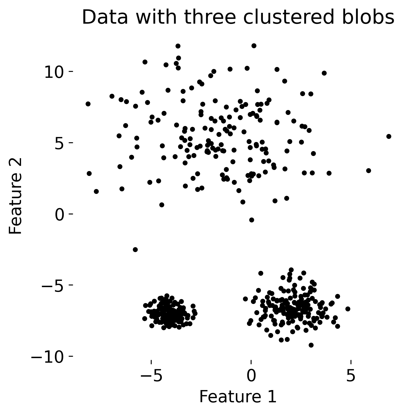
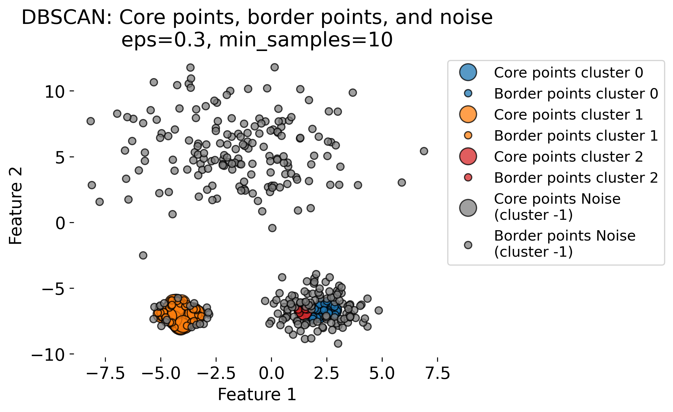
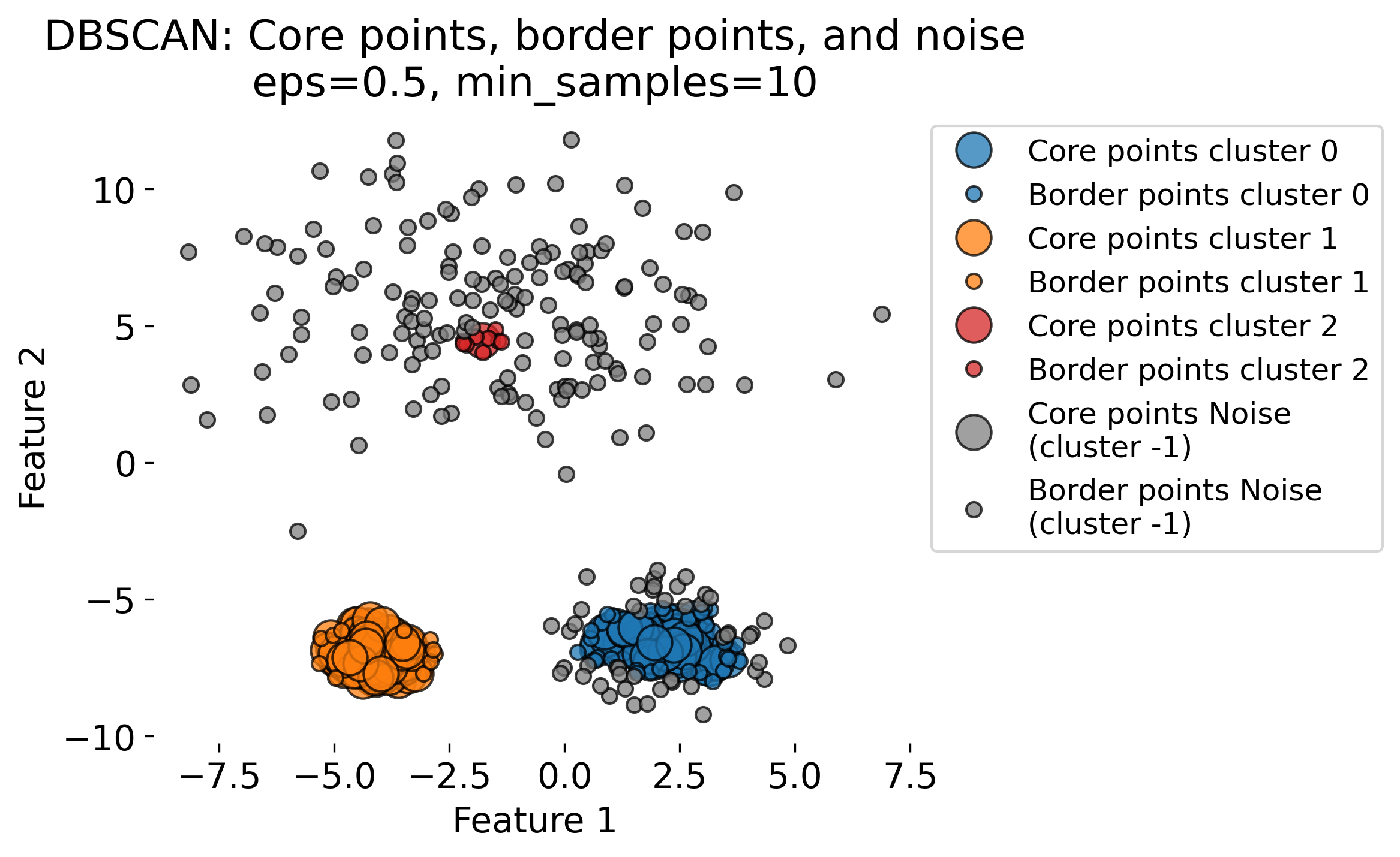
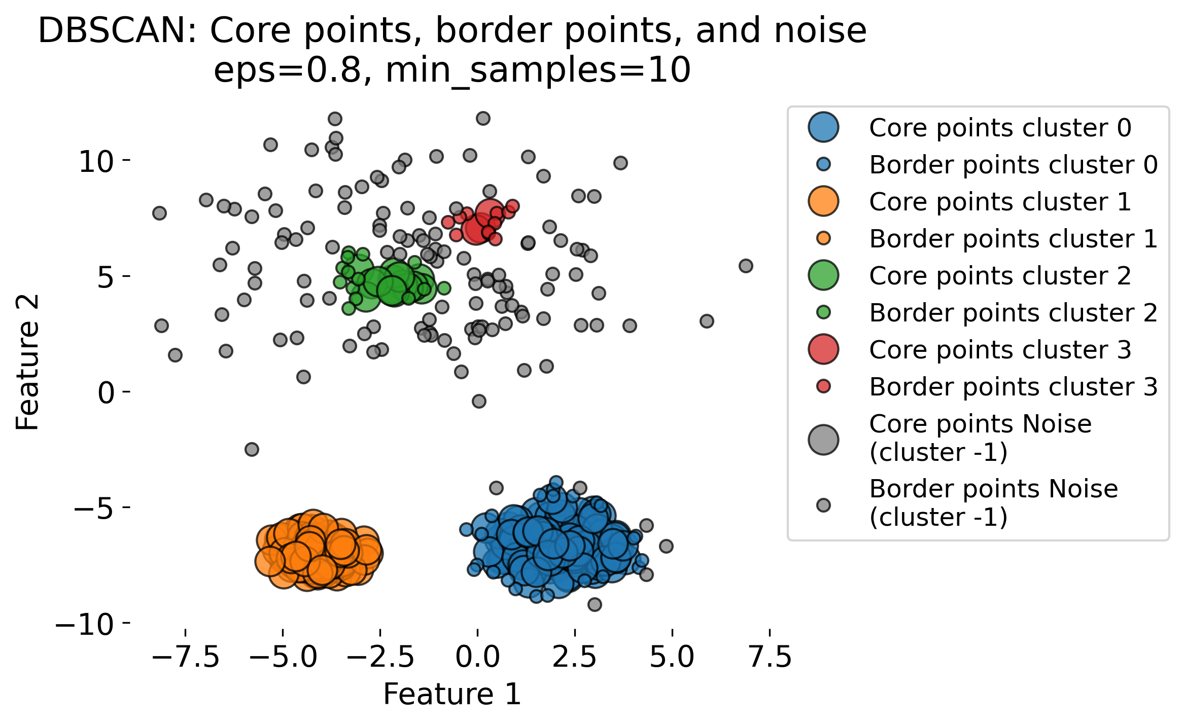
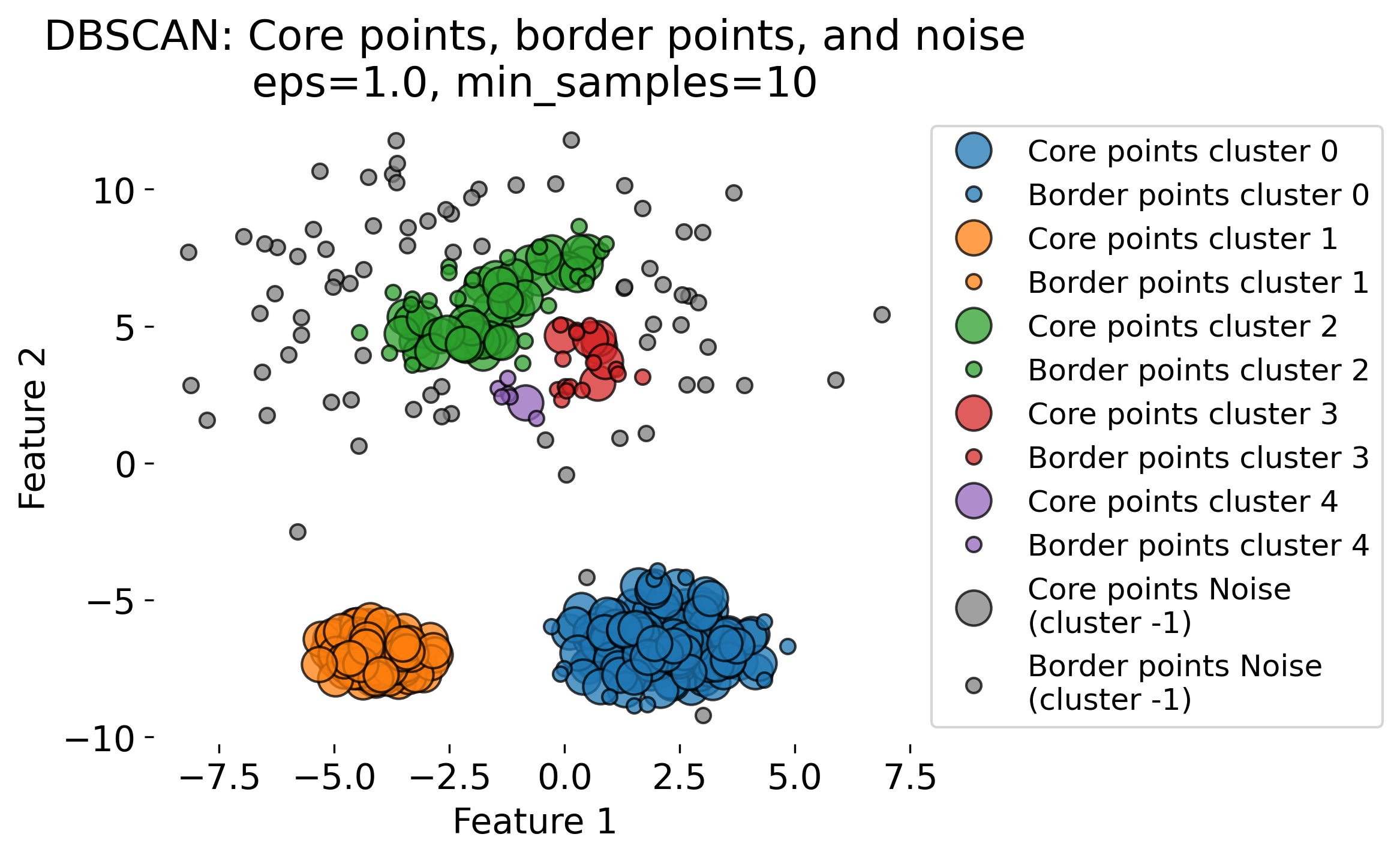
The figure demonstrates the DBSCAN (Density-Based Spatial Clustering of Applications with Noise) algorithm applied to a dataset with three clusters (blobs, each having different standard deviations). DBSCAN is a density-based clustering algorithm that identifies clusters based on two key parameters: the radius (epsilon or eps) and the minimum number of points (min_samples) required to form a dense region. The algorithm classifies data points into three categories: 1. Core Points: Points that have at least min_samples neighbors within the radius eps. These are central points in high-density regions (by evaluating the local density around each data point based on these two key parameters). 2. Border Points: Points that fall within the eps radius of a core point but do not have enough neighbors themselves to be core points. 3. Noise Points: Points that do not belong to any cluster, often isolated or in low-density regions.
The plots show the results of DBSCAN with different eps values (eps = 0.3, 0.5, 0.8, 1.0). Small eps values (e.g., 0.3) result in more noise points (shown in gray) and smaller clusters, as the algorithm is more conservative in grouping points. Larger eps values (e.g., 1.0) allow DBSCAN to group more points into clusters, sometimes resulting in fewer, larger clusters. As eps increases, more points are classified as core points and fewer as noise.
These variations highlight the sensitivity of DBSCAN to the eps parameter. DBSCAN excels at identifying clusters of arbitrary shapes and densities, unlike traditional algorithms like k-means.

Algorithm overview

1. Neighborhood query

For each point $x_i$, find its $\epsilon$-neighborhood, defined as:

\[N_{\epsilon}(x_i) = \{ x_j \in X : d(x_i, x_j) \leq \epsilon \}\]

This set contains all points within a distance $\epsilon$ from $x_i$.

2. Core point identification

A point $x_i$ is identified as a core point if:

\[|N_{\epsilon}(x_i)| \geq \text{MinPts}\]

If $x_i$ satisfies this condition, it becomes the starting point for a new cluster.

3. Cluster formation

Starting from each core point, a cluster is formed by recursively expanding the $\epsilon$-neighborhood to include all directly or indirectly reachable points. A point $x_j$ is reachable from a core point $x_i$ if there exists a chain of core points $x_1, x_2, \dots, x_j$ such that:

\[d(x_i, x_1) \leq \epsilon, \; d(x_1, x_2) \leq \epsilon,\] \[\dots, \; d(x_{j-1}, x_j) \leq \epsilon\]

Border points, which lie within the $\epsilon$-neighborhood of core points but do not have enough neighbors themselves to be core points, are added to the nearest cluster.

4. Noise identification

Any point that is not reachable from any core point (i.e., neither a core nor a border point) is labeled as noise.

DBSCAN parameters

• $\epsilon$: The radius that defines the neighborhood around each point. A larger $\epsilon$ results in fewer but larger clusters, while a smaller $\epsilon$ leads to more, smaller clusters.
• $\text{MinPts}$: The minimum number of points required to form a dense region. Typically, $\text{MinPts}$ is set to 4 or higher, depending on the dataset.

Advantages and limitations of DBSCAN

Advantages:

• Non-Parametric: Unlike k-Means, DBSCAN does not require specifying the number of clusters in advance.
• Arbitrary-Shaped Clusters: Can identify clusters of arbitrary shapes.
• Robust to Noise: Able to handle noise and outliers.

Limitations:

• Parameter Sensitivity: The results of DBSCAN are sensitive to the choice of $ \epsilon $ and $ MinPts $.
• Varying Densities: Struggles with datasets that contain clusters of widely varying densities.

Computational complexity

The time complexity of DBSCAN is $O(n^2)$, but this can be reduced to $O(n \log n)$ with efficient indexing structures such as kd-trees (k-dimensional tree, a data structure used for organizing points in a k-dimensional space; it is a binary search tree that recursively partitions the space into two half-spaces by hyperplanes).

Python example

In its simplest form, DBSCAN can be performed by executing two lines of Python code:

circles_data = datasets_all[0] # select the circles dataset

# set DBSCAN parameters:
eps = 0.2
min_samples = 10

# create the DBSCAN object:
dbscan = cluster.DBSCAN(eps=eps, min_samples=min_samples)

# fit the data:
dbscan_fit = dbscan.fit(circles_data[0])

Check whether the clustering results are as expected (should have the same shape as the data):

print(f"shape of the data: {circles_data[0].shape}")
print(f"shape of the labels: {dbscan_fit.labels_.shape}")

shape of the data: (500, 2)
shape of the labels: (500,)

And plot the clustering results:

fig, ax = plt.subplots(1, 1, figsize=(5, 5))
ax.scatter(circles_data[0][:, 0], circles_data[0][:, 1], c=dbscan_fit.labels_, s=10)
ax.set_title(f'DBSCAN clustering (eps={eps},\nmin_samples={min_samples})')
plt.show()

DBSCAN clustering results (right) with $\epsilon=0.2$ and $\text{MinPts}=10$ on the circles dataset (left).

Here are the results for all datasets:

DBSCAN clustering results with $\epsilon=0.3$ and $\text{MinPts}=10$ on all datasets.

Comparison of clustering methods

• k-Means is fast and simple but requires specifying the number of clusters and assumes spherical clusters.
• Agglomerative clustering is versatile, as it doesn’t require pre-specifying the number of clusters and can handle complex shapes, but it is computationally expensive.
• DBSCAN excels in identifying clusters of arbitrary shapes and is robust to noise, but its performance is highly sensitive to parameter choices and struggles with clusters of varying densities.

Each method has its own strengths and limitations, and the choice of algorithm depends on the specific characteristics of the dataset and the goals of the analysis.

Summary of different clustering methods applied to various datasets.

k-means, agglomerative clustering, and DBSCAN are just a few examples of clustering algorithms, exemplarily chosen to illustrate different approaches to clustering. There are many other clustering algorithms available, each with its own characteristics and use cases. For instance, scikit-learn’s modeul sklearn.cluster provides a wide range of clustering algorithms that can be applied to various datasets.

Exercise

In the exercise, you will explore the three clustering methods presented above (k-Means, Agglomerative clustering, and DBSCAN) applied to neural data (calcium imaging data from a mouse; similar to the PCA chapter). You will experiment with different parameter settings and observe how the clustering results change. Additionally, you will evaluate the clustering results using the silhouette score and silhouette plots.

Agglomerative clustering applied to the PCA of a high-dimensional neural dataset.

Access the exercise notebook here: