Campbell and Siegert approximation for estimating the firing rate of a neuron

The Campbell and Siegert approximation is a method used in computational neuroscience to estimate the firing rate of a neuron given a certain input. This approximation is particularly useful for analyzing the firing behavior of neurons that follow a leaky integrate-and-fire (LIF) model or similar models under the influence of stochastic input currents.

Spike raster plot and histogram of the spiking rate of a neuron receiving Poisson spike trains as input. Included are the actual firing rate and the estimated firing rate using the Campbell & Siegert approximation. Further explanations can be found in the text below.

Mathematical foundations

The Campbell and Siegert approximation combines Campbell’s theorem with Siegert’s analysis of the so-called first-passage time problem.

Campbell’s theorem

Campbell’s theorem states that the mean and variance of the summed input to a neuron driven by a Poisson process can be derived from the properties of the individual inputs. In general, for a point process $N$ defined on an $n$-dimensional Euclidean space $\textbf{R}^n$, Campbell’s theorem offers a way to calculate the expected value of a function $f$ of the point process $N$ as

\[\operatorname{E} \left[\sum _{x\in N}f(x)\right]=\int _{\textbf{R}^n}f(x)\Lambda (dx)\]

where the sum is over all points in the point process. $\operatorname{E}$ denotes the expectation operator, and $\Lambda$ is the intensity measure of the point process:

\[\Lambda(B) = E\left[N(B)\right]\]

where $N(B)$ is the number of points in the set $B$. $B$ can be any Borel set (any set that can be formed from open sets through the operations of countable union, countable intersection, and relative complement) in $\textbf{R}^n$.

Given a neuron receiving synaptic inputs from Poisson-distributed spike trains, Campbell’s theorem can be used to calculate the mean input current $\mu$:

\[\mu = \sum_{i=1}^{N} w_i \lambda_i\]

where $w_i$ is the synaptic weight of the $i$-th synapse and $\lambda_i$ is the firing rate of the $i$-th presynaptic neuron, i.e., the rate of the Poisson process from input $i$. For a large number of inputs with similar properties, this sum becomes:

\[\mu = N \cdot w \cdot \lambda\]

where $N$ is the number of inputs, $w$ is the average synaptic weight, and $\lambda$ is the average rate of the presynaptic neurons (or Poisson input). The variance $\sigma^2$ of the input current can be calculated accordingly:

\[\sigma^2 = \sum_{i=1}^{N} w_i^2 \lambda_i\]

Similarly, for a large number of similar inputs we have:

\[\sigma^2 = N \cdot w^2 \cdot \lambda\]

Siegert’s approximation

Siegert’s approximation (Siegert 1950ꜛ) on the other hand is used to estimate the firing rate of a neuron by considering the dynamics of the membrane potential and the first-passage time (the time it takes for the membrane potential to reach the threshold for the first time). This involves solving an integral that describes the distribution of first-passage times, which is influenced by the mean and variance of the input current:

\[\nu \approx \frac{\mu - V_{\text{reset}}}{\Delta V} \exp\left(\frac{\mu^2}{2\sigma^2}\right)\]

where:

• $\nu$ is the firing rate of the neuron that is being estimated
• $\mu$ is the mean input current which can be calculated using Campbell’s theorem
• $\sigma^2$ is the variance of the input current, also calculated using Campbell’s theorem
• $V_{\text{reset}}$ is the reset potential of the neuron
• $\Delta V$ is the difference between the threshold potential and the reset potential.

The exponential term captures the effect of the input variance on the firing rate. The term $\frac{\mu - V_{\text{reset}}}{\Delta V}$ normalizes the firing rate to the range between 0 and 1.

The equation above is what is known as the Campbell & Siegert approximation, which provides a simple and effective way to estimate the firing rate of a neuron based on the mean and variance of the input current. This approximation is particularly useful for understanding the behavior of neurons in response to fluctuating inputs and is commonly used in theoretical neuroscience and computational modeling. It simplifies the complex dynamics of the LIF model under stochastic inputs to a more manageable form. However, the approximation has its limitations, especially when the input statistics deviate significantly from the assumptions of the model.

Example

The will replicate the NEST tutorial “Campbell & Siegert approximation example”ꜛ with some modifications in order to calculate the firing rate of a neuron based on the mean and variance of the input current. We will then compare the estimated firing rate with the actual firing rate simulated with the NEST simulator.

Let’s first import the necessary libraries and define the parameters for the simulation:

import os
import matplotlib.pyplot as plt
import matplotlib.gridspec as gridspec
import numpy as np
from scipy.optimize import fmin
from scipy.special import erf
import nest
import nest.raster_plot

# set global properties for all plots:
plt.rcParams.update({'font.size': 12})
plt.rcParams["axes.spines.top"]    = False
plt.rcParams["axes.spines.bottom"] = False
plt.rcParams["axes.spines.left"]   = False
plt.rcParams["axes.spines.right"]  = False

# set the simulation time:
simtime = 20000  # (ms) duration of simulation

# define some units:
pF = 1e-12
ms = 1e-3
pA = 1e-12
mV = 1e-3

# set the parameters of the neurons and noise sources:
n_neurons = 10  # number of simulated neurons

weights = [0.1]  # (mV) psp amplitudes
rates = [10000.0]  # (1/s) rate of Poisson sources
# weights = [0.1, 0.1]    # (mV) psp amplitudes
# rates = [5000., 5000.]  # (1/s) rate of Poisson sources

C_m     = 250.0  # (pF) capacitance
E_L     = -70.0  # (mV) resting potential
I_e     = 0.0  # (nA) external current
V_reset = -70.0  # (mV) reset potential
V_th    = -55.0  # (mV) firing threshold
t_ref   = 2.0  # (ms) refractory period
tau_m   = 10.0  # (ms) membrane time constant
tau_syn_ex = 0.5  # (ms) excitatory synaptic time constant
tau_syn_in = 2.0  # (ms) inhibitory synaptic time constant

Next, we analytically calculate the mean and variance of the input current using the Campbell theorem:

# estimate the mean and variance of the input current using the Campbell & Siegert approximation:
mu = 0.0
sigma2 = 0.0
J = []
assert len(weights) == len(rates)
for rate, weight in zip(rates, weights):
    if weight > 0:
        tau_syn = tau_syn_ex
    else:
        tau_syn = tau_syn_in

    # we define the form of a single PSP (post-synaptic potential), which allows us to match the
    # maximal value to or chosen weight:
    def psp(x):
        return -(
            (C_m * pF)
            / (tau_syn * ms)
            * (1 / (C_m * pF))
            * (np.exp(1) / (tau_syn * ms))
            * (
                ((-x * np.exp(-x / (tau_syn * ms))) / (1 / (tau_syn * ms) - 1 / (tau_m * ms)))
                + (np.exp(-x / (tau_m * ms)) - np.exp(-x / (tau_syn * ms)))
                / ((1 / (tau_syn * ms) - 1 / (tau_m * ms)) ** 2)
            )
        )

    min_result = fmin(psp, [0], full_output=1, disp=0)

    # we need to calculate the PSC amplitude (i.e., the weight we set in NEST)
    # from the PSP amplitude, that we have specified above:
    fudge = -1.0 / min_result[1]
    J.append(C_m * weight / (tau_syn) * fudge)

    # we now use Campbell's theorem to calculate mean and variance of the input 
    # due to the Poisson sources. The mean and variance add up for each Poisson source:
    mu += rate * (J[-1] * pA) * (tau_syn * ms) * np.exp(1) * (tau_m * ms) / (C_m * pF)
    sigma2 += (
        rate
        * (2 * tau_m * ms + tau_syn * ms)
        * (J[-1] * pA * tau_syn * ms * np.exp(1) * tau_m * ms / (2 * (C_m * pF) * (tau_m * ms + tau_syn * ms))) ** 2
    )

mu += E_L * mV          # add the resting potential and convert to mV
sigma = np.sqrt(sigma2) # convert the variance to standard deviation

After calculating the mean and variance of the input current, we can now calculate the firing rate using Siegert’s approximation:

num_iterations = 100 # number of iterations for the integral
upper = (V_th * mV - mu) / (sigma * np.sqrt(2))
lower = (E_L * mV - mu) / (sigma * np.sqrt(2))
interval = (upper - lower) / num_iterations
tmpsum = 0.0
for cu in range(0, num_iterations + 1):
    u = lower + cu * interval
    f = np.exp(u**2) * (1 + erf(u))
    tmpsum += interval * np.sqrt(np.pi) * f
r = 1.0 / (t_ref * ms + tau_m * ms * tmpsum) # firing rate

r is the estimated firing rate of the neuron based on the mean and variance of the input current.

We can now simulate the neurons receiving Poisson spike trains as input and compare the theoretical firing rate with the empirical value:

nest.set_verbosity("M_WARNING")
nest.ResetKernel()

# define the parameters of the neurons for NEST:
neurondict = {
    "V_th": V_th,
    "tau_m": tau_m,
    "tau_syn_ex": tau_syn_ex,
    "tau_syn_in": tau_syn_in,
    "C_m": C_m,
    "E_L": E_L,
    "t_ref": t_ref,
    "V_m": E_L,
    "V_reset": E_L,
}

# create the neurons, Poisson generators, voltmeter, and spike recorder:
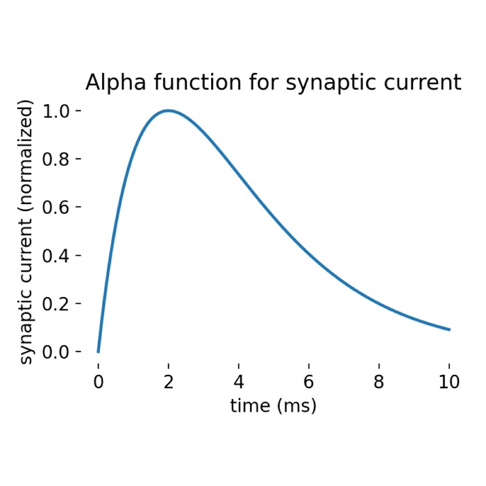
neurons     = nest.Create("iaf_psc_alpha", n_neurons, params=neurondict) 
neuron_free = nest.Create("iaf_psc_alpha", params=dict(neurondict, V_th=1e12))
poissongen    = nest.Create("poisson_generator", len(rates), {"rate": rates})
voltmeter     = nest.Create("voltmeter", params={"interval": 0.1})
spikerecorder = nest.Create("spike_recorder")

# connect the nodes:
poissongen_n_synspec = {"weight": np.tile(J, ((n_neurons), 1)), "delay": 0.1}
nest.Connect(poissongen, neurons, syn_spec=poissongen_n_synspec)
nest.Connect(poissongen, neuron_free, syn_spec={"weight": [J]})
nest.Connect(voltmeter, neuron_free)
nest.Connect(neurons, spikerecorder)

# simulate the network:
nest.Simulate(simtime)

In the simulation code above, we create a network of 10 neurons receiving Poisson spike trains as input. The neurons are modelled using the iaf_psc_alpha neuron model, which is a leaky integrate-and-fire model with alpha-shaped postsynaptic currents. We create an additional neuron neuron_free with a very high threshold potential, which prevents it from spiking and, thus, making a ‘silent’ neuron. This allows to record the membrane potential without the neuron spiking. We also record the spike times of the neurons to calculate the empirical firing rate.

Finally, we plot the membrane potential of the silent neuron,

# extract the membrane potential of the silent neuron:
v_free = voltmeter.events["V_m"]
Nskip = 500 # we skip the first 500 ms of the simulation

# plot the membrane potential of the silent neuron:
plt.figure(figsize=(6, 4))
plt.plot(voltmeter.events["times"][Nskip:], v_free[Nskip:], label=f"membrane potential $V_m$")
plt.axhline(y=V_th, color='r', linestyle='--', label=f"threshold potential $V_$")
plt.axhline(y=V_reset, color='g', linestyle='--', label=f"reset potential $V_$")
plt.xlabel("time [ms]")
plt.ylabel("membrane potential [mV]")
plt.ylim([-71, -51])
plt.legend()
plt.title("Membrane potential of silent neuron")
plt.tight_layout()
plt.savefig("figures/campbell_siegert_approximation_membrane_potential.png", dpi=300)
plt.show()

and the spike raster plot with the histogram of the spiking rate:

# extract the spike times and neuron IDs:
spike_events = nest.GetStatus(spikerecorder, "events")[0]
spike_times = spike_events["times"]
neuron_ids = spike_events["senders"]

# combine the spike times and neuron IDs into a single array and sort by time:
spike_data = np.vstack((spike_times, neuron_ids)).T
spike_data_sorted = spike_data[spike_data[:, 0].argsort()]

# extract sorted spike times and neuron IDs:
sorted_spike_times = spike_data_sorted[:, 0]
sorted_neuron_ids = spike_data_sorted[:, 1]

# spike raster plot and histogram of spiking rate ("manually" plotted):
fig = plt.figure(figsize=(6, 6))
gs = gridspec.GridSpec(5, 1)

# create the first subplot (3/4 of the figure)
ax1 = plt.subplot(gs[0:4, :])
ax1.scatter(sorted_spike_times, sorted_neuron_ids, s=9.0, color='mediumaquamarine', alpha=1.0)
ax1.set_title(f"Spike raster plot and histogram of spiking rate")
#ax1.set_xlabel("time [ms]")
ax1.set_xticks([])
ax1.set_ylabel("neuron ID")
ax1.set_xlim([0, simtime])
ax1.set_ylim([0, n_neurons+1])
ax1.set_yticks(np.arange(0, n_neurons+1, 10))

# create the second subplot (1/4 of the figure)
ax2 = plt.subplot(gs[4, :])
hist_binwidth = 55.0
t_bins = np.arange(np.amin(sorted_spike_times), np.amax(sorted_spike_times), hist_binwidth)
n, bins = np.histogram(sorted_spike_times, bins=t_bins)
heights = 10000 * n / (hist_binwidth * (n_neurons))
ax2.bar(t_bins[:-1], heights, width=hist_binwidth, color='violet')
#ax2.set_title(f"histogram of spiking rate vs. time")
ax2.text(0.05, 0.95, f"calculated firing rate: {np.round(r,2)} Hz",
            color='black', fontsize=12, ha='left', va='center',
            transform=plt.gca().transAxes, bbox=dict(facecolor='white', edgecolor='white', alpha=0.5))
ax2.text(0.05, 0.7, f"actual firing rate:        {np.round(spikerecorder.n_events/(n_neurons * simtime * ms),2)} Hz", 
         color='black', fontsize=12, ha='left', va='center', 
         transform=plt.gca().transAxes, bbox=dict(facecolor='white', edgecolor='white', alpha=0.5))
ax2.set_ylabel("firing rate\n[Hz]")
ax2.set_xlabel("time [ms]")
ax2.set_xlim([0, simtime])

plt.tight_layout()
plt.show()

To compare the estimated firing rate with the actual firing rate, we can calculate the empirical firing rate from the spike times of the neurons:

print(f"mean membrane potential (actual / calculated): {np.mean(v_free[Nskip:])} / {mu * 1000}")
print(f"variance (actual / calculated): {np.var(v_free[Nskip:])} / {sigma2 * 1e6}")
print(f"firing rate (actual / calculated): {spikerecorder.n_events / (n_neurons * simtime * ms)} / {r}")

mean membrane potential (actual / calculated): -57.79420883300154 / -57.81894163122827
variance (actual / calculated): 0.6809326908771234 / 0.6897398528707916
firing rate (actual / calculated): 0.185 / 0.2898135046747145

The estimated firing rate using the Campbell & Siegert approximation is 0.29 Hz, while the empirical firing rate is 0.185 Hz. The membrane potential and variance are also close to the theoretical values calculated using the mean and variance of the input current. The discrepancy between the estimated and empirical firing rates can be attributed to the simplifying assumptions made in the approximation.

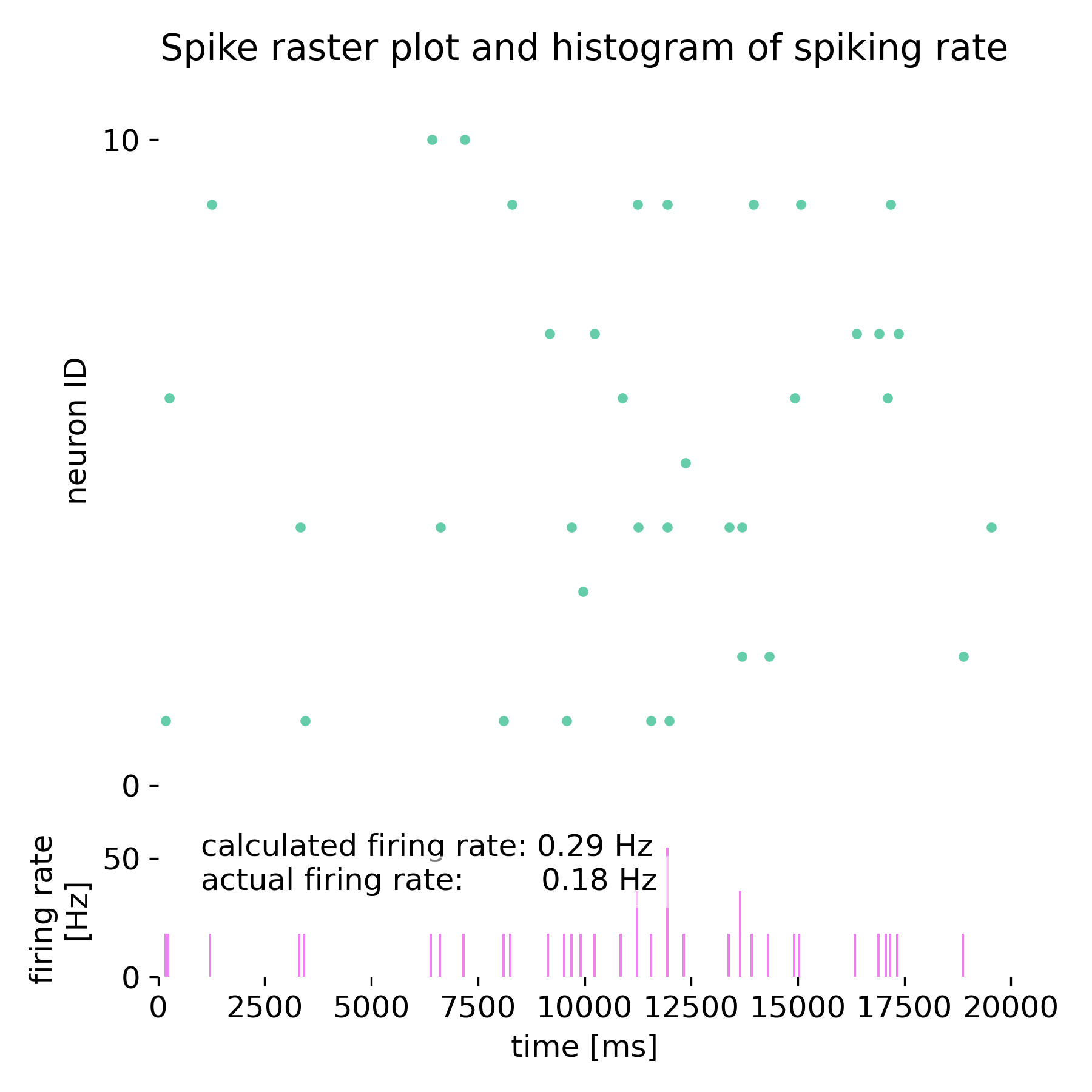
Spike raster plot and histogram of spiking rate for the 10 neurons simulated in NEST, receiving Poisson spike trains as input.

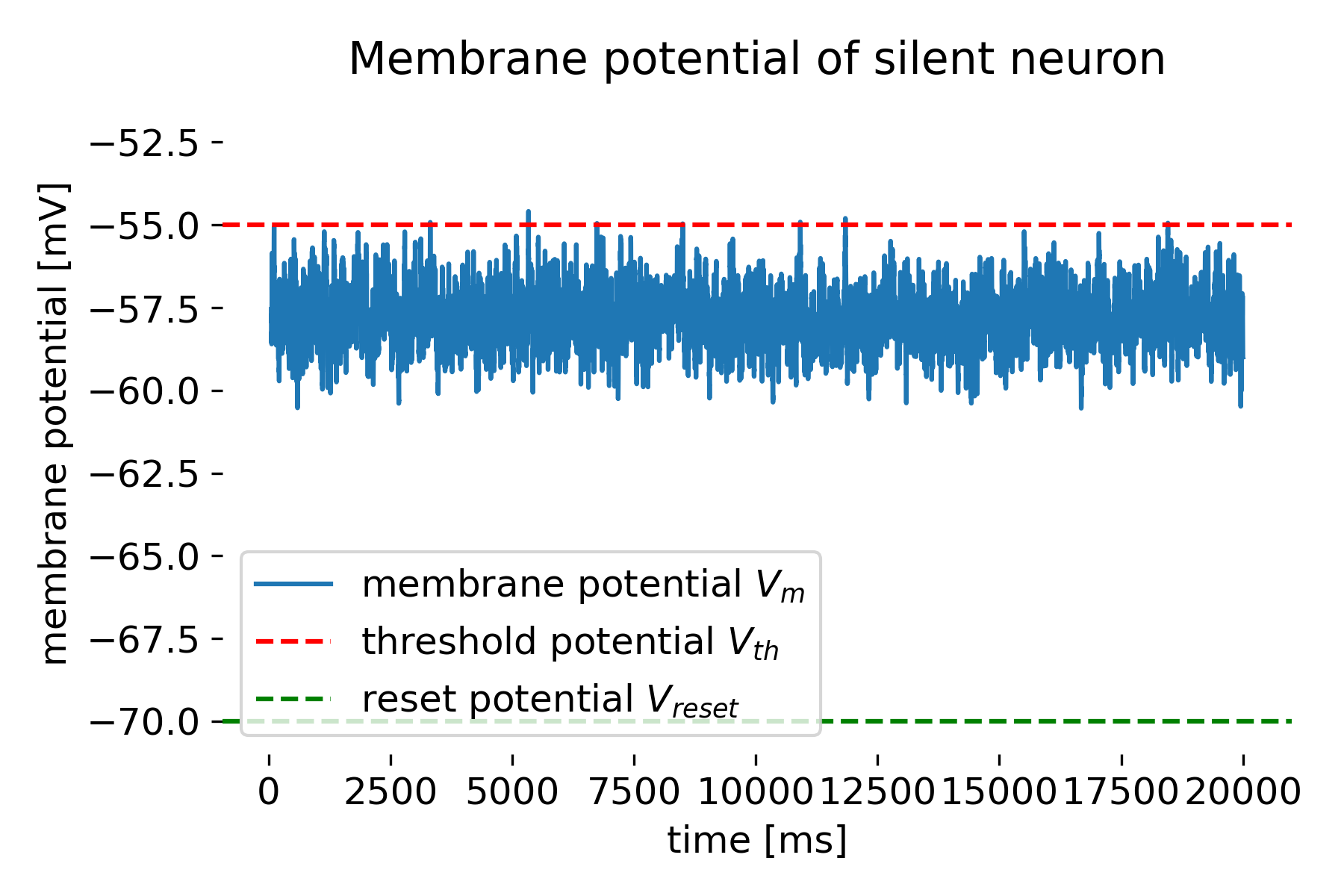
Membrane potential of the modelled silent neuron.

Conclusion

The Campbell and Siegert approximation is a valuable tool for estimating the firing rate of neurons in models where the input is stochastic. By using the mean and variance of the input current, this approximation provides insights into how neurons might respond to varying synaptic inputs, making it a crucial concept in the study of neural coding and information processing in computational neuroscience.

The complete code used in this blog post is available in this Github repositoryꜛ (campbell_siegert_approximation.py). Feel free to modify and expand upon it, and share your insights.

References and useful links

• Wikipedia article on Campbell’s theoremꜛ
• Siegert, On the First Passage Time Probability Problem, 1950, Physical Review, Vol. 81, Issue 4, pages 617-623, doi: 10.1103/PhysRev.81.617ꜛ
• Athanasios Papoulis, S. Unnikrishna Pillai, Probability, Random Variables, And Stochastic Processes, 2002, McGraw-Hill Companies, ISBN: 9780071122566
• Florian Jug, Matthew Cook, Angelika Steger, Recurrent competitive networks can learn locally excitatory topologies, 2012, The 2012 International Joint Conference on Neural Networks (IJCNN), doi: 10.1109/IJCNN.2012.6252786ꜛ
• Luigi M. Ricciardi, Charles E. Smith, Diffusion Processes And Related Topics In Biology, 1977, Springer, ISBN: 9783540081463, source-urlꜛ
• Ostojic, S, & Brunel, N, From [spiking neuron models to linear-nonlinear models (2011), PLoS Comput Biol, 7(1), e1001056. doi: 10.1371/journal.pcbi.1001056ꜛ
• NEST tutorial “Campbell & Siegert approximation example”ꜛ