Exponential (EIF) and adaptive exponential Integrate-and-Fire (AdEx) model

The exponential Integrate-and-Fire (EIF) model is a simplified neuronal model that captures the essential dynamics of action potential generation. It extends the classical Integrate-and-Fire (IF) model by incorporating an exponential term to model the rapid rise of the membrane potential during spike initiation more accurately. The adaptive exponential Integrate-and-Fire (AdEx) model is a variant of the EIF model that includes an adaptation current to account for spike-frequency adaptation observed in real neurons. In this tutorial, we will explore the key features of the EIF and AdEx models and their applications in simulating neuronal dynamics.

Mathematical foundations

We will first derive the exponential Integrate-and-Fire (EIF) model from the Hodgkin-Huxley model. Let’s therefore recall the Hodgkin-Huxley (HH) model and its key equations. The HH model uses four coupled nonlinear differential equations to represent the dynamics of the membrane potential and the three gating variables of sodium ($\text{Na}^+$) and potassium ($\text{K}^+$) ion channels. The membrane potential is given by:

\[C \frac{dV}{dt} = I_{\text{ext}} - \left( I_{\text{Na}} + I_{\text{K}} + I_{\text{leak}} \right)\]

where

• $V$ is the membrane potential
• $C$ is the membrane capacitance
• $I_{\text{ext}}$ is the external input current
• $I_{\text{Na}}$, $I_{\text{K}}$, and $I_{\text{leak}}$ are the sodium, potassium, and leak currents, respectively.

The ionic currents are described by:

\[\begin{align*} I_{\text{Na}} &= g_{\text{Na}} m^3 h (V - E_{\text{Na}}) \\ I_{\text{K}} &= g_{\text{K}} n^4 (V - E_{\text{K}}) \\ I_{\text{leak}} &= g_{\text{leak}} (V - E_{\text{leak}}) \end{align*}\]

The gating variables $m$, $h$, and $n$ follow first-order kinetics:

\[\begin{align*} \frac{dm}{dt} &= \alpha_m (1 - m) - \beta_m m \\ \frac{dh}{dt} &= \alpha_h (1 - h) - \beta_h h \\ \frac{dn}{dt} &= \alpha_n (1 - n) - \beta_n n \end{align*}\]

Derivation of the EIF model

The EIF model was first introduced by Nicolas Fourcaud-Trocmé et al. in 2003ꜛ. To derive the model, several approximations and simplifications are applied to the Hodgkin-Huxley model. First, the dynamics of the gating variables are assumed to be much faster than the changes in the membrane potential, allowing us to approximate them by their quasi-steady states. Second, focusing on the rapid rise of the membrane potential during an action potential, the sodium current can be approximated by an exponential function of the membrane potential. This is because the activation of sodium channels increases rapidly with voltage. Let’s therefore approximate the sodium current as:

\[I_{\text{Na}} \approx g_L \Delta_T \exp \left( \frac{V - V_T}{\Delta_T} \right)\]

where $V_T$ is the threshold potential, $g_L$ is the leak conductance, and $\Delta_T$ is the slope factor.

The leak current remains linear and is given by:

\[I_{\text{leak}} = g_L (V - E_L)\]

where $E_L$ is the leak reversal potential.

Combining the approximations for the ionic currents, the total membrane current is:

\[\begin{align*} I_{\text{total}} =& \quad 6 g_L (E_L - V) \\ &+ g_L \Delta_T \exp \left( \frac{V - V_T}{\Delta_T} \right) + I_{\text{ext}} \end{align*}\]

Using the membrane capacitance $C$, the equation for the membrane potential $V$ becomes:

\[\begin{align*} C \frac{dV}{dt} =& -g_L (V - E_L) \\ &+ g_L \Delta_T \exp \left( \frac{V - V_T}{\Delta_T} \right) + I_{\text{ext}} \end{align*}\]

This is the core equation of the EIF model. Once the membrane potential reaches the threshold $V_T$, a spike is generated, and the membrane potential is reset to a reset value $V_{\text{reset}}$:

\[\text{if } V \geq V_{\text{T}} \text{ then } V \leftarrow V_{\text{reset}}\]

Derivation of the AdEx model

The adaptive exponential Integrate-and-Fire (AdEx or AEIF) model was first introduced by Romain Brette and Wulfram Gerstner in 2005ꜛ. It builds upon the EIF model by incorporating an adaptation current to account for the spike-frequency adaptation observed in real neurons. This adaptation mechanism is crucial for modeling the neuron’s ability to adjust its firing rate in response to prolonged stimulation. The adaptation current $w$ represents the slow adaptation mechanism and is modeled as a function of the membrane potential:

\[\tau_w \frac{dw}{dt} = a (V - E_L) - w\]

where

• $\tau_w$ is the adaptation time constant, and
• $a$ is the subthreshold adaptation parameter.

The membrane potential equation in the AdEx model is similar to the EIF model but incorporates the adaptation current $w$:

\[\begin{align*} C \frac{dV}{dt} &= -g_L (V - E_L) \\ &+ g_L \Delta_T \exp \left( \frac{V - V_T}{\Delta_T} \right) \\ &- w + I_{\text{ext}} \\ \end{align*}\]

As for the Hodgkin-Huxley model, the AdEx model can include additional conductances and currents to capture specific neuronal properties. For instance, an excitatory synaptic conductance $g_\text{ex}$ and an inhibitory synaptic conductance $g_\text{in}$ can be added to model synaptic inputs:

\[\begin{align*} C \frac{dV}{dt} =& -g_L (V - E_L) \\ &+ g_L \Delta_T \exp \left( \frac{V - V_T}{\Delta_T} \right)\\ & - g_\text{ex} (V - E_\text{ex}) \\ &- g_\text{in} (V - E_\text{in}) - w + I_{\text{ext}} \end{align*}\]

Once a spike occurs, the membrane potential is reset to a reset value $V_{\text{reset}}$, and the adaptation current is increased by an amount $b$, the spike-triggered adaptation parameter, as each spike causes a jump in the adaptation current:

\[\text{if } V \geq V_{\text{T}} \text{ then } \begin{cases} V \leftarrow V_{\text{reset}} \\ w \leftarrow w + b \end{cases}\]

where

• $V_{\text{th}}$ is the threshold potential, and
• $b$ is the spike-triggered adaptation parameter.

Applications of EIF and AdEx Models

The EIF and AdEx models are widely used in computational neuroscience for their balance between biological realism and computational efficiency. Here are a few applications:

Large-scale neuronal network simulations

These models are computationally efficient and can be used to simulate large networks of spiking neurons, making them suitable for studying network dynamics, such as oscillations, synchronization, and information processing in the brain.

Understanding neuronal response properties

The models help to understand how neurons respond to different input currents and how various parameters affect the firing patterns, such as spike-frequency adaptation in the AdEx model.

Comparison with experimental data

These models provide a framework to compare theoretical predictions with experimental data, helping to refine our understanding of the underlying mechanisms of neuronal behavior.

Simulating the AdEx model in Python

To simulate the AdEx model in Python, we can use the aief_cond_alphaꜛ neuron model implemented in the NEST simulator. We will create an AdEx neuron with multiple DC inputs, one with a lower amplitude of 500 pA lasting from 0 to 200 ms and another with a higher amplitude of 800 pA lasting from 500 to 1000 ms. We will also record the membrane potential using a voltmeter. We will use a subthreshold adaptation parameter of $a=4.0$ and a spike-triggered adaptation parameter $b=80.5$ to reproduce figure 2C from the original AdEx model paper by Brette and Gerstner (2005)ꜛ. The following Python code is adapted and slightly modified from the NEST tutorial “Testing the adapting exponential integrate and fire model in NEST (Brette and Gerstner Fig 2C)”ꜛ

import os
import matplotlib.pyplot as plt
import nest

# set global properties for all plots:
plt.rcParams.update({'font.size': 12})
plt.rcParams["axes.spines.top"]    = False
plt.rcParams["axes.spines.bottom"] = False
plt.rcParams["axes.spines.left"]   = False
plt.rcParams["axes.spines.right"]  = False

nest.set_verbosity("M_WARNING")
nest.ResetKernel()

# set the simulation and the resolution of the simulation:
T = 1000.0 # ms
nest.resolution = 0.1 # ms

# create an AEIF neuron with multiple synapses:
neuron = nest.Create("aeif_cond_alpha")

# set the parameters of the AEIF neuron:
neuron.set(a=4.0, b=80.5)

# create two DC generators:
dc = nest.Create("dc_generator", 2)
dc.set(amplitude=[500.0, 800.0], start=[0.0, 500.0], stop=[200.0, 1000.0])

# connect the DC generators to the neuron:
nest.Connect(dc, neuron, "all_to_all")

# create a voltmeter to record the membrane potential of the neuron:
voltmeter = nest.Create("voltmeter", params={"interval": 0.1})
nest.Connect(voltmeter, neuron)

# simulate the network:
nest.Simulate(T)

# extract the data from the voltmeter:
Vms  = voltmeter.get("events", "V_m")
time = voltmeter.get("events", "times")

# plot the membrane potential:
plt.figure(figsize=(5.5, 4))
plt.plot(time, Vms)
plt.xlabel("time (ms)")
plt.ylabel("membrane potential (mV)")
plt.title(f"AdEx neuron with multiple DC inputs")
plt.grid(True)
plt.tight_layout()
plt.show()

Membrane potential of an AdEx neuron modelled with multiple DC inputs.

From the simulation results, we can distinguish three phases in the membrane potential trace:

1. Initial phase (0-200 ms): The neuron receives a DC input of 500 pA, which is below the threshold needed to generate spikes. This phase shows subthreshold activity with a small depolarization and possible overshoot due to the subthreshold adaptation mechanism.
2. Intermediate phase (200-500 ms): There is no DC input, so the membrane potential returns closer to the resting potential.
3. Late phase (500-1000 ms): The neuron receives a stronger DC input of 800 pA, which is above the threshold, leading to spiking activity. The spike frequency is high initially but decreases over time due to the spike-triggered adaptation, demonstrating the characteristic spike-frequency adaptation of the AdEx model.

These observations align well with the expected behavior of the AdEx model as described in the original paper by Brette and Gerstnerꜛ.

AdEx model with multiple synapses and synaptic dynamics

NEST holds a variant of the aeif_cond_alpha model called aeif_cond_beta_multisynapseꜛ that allows for an AdEx model with multiple synapses with different synaptic dynamics. The following Python code demonstrates how to create such a model and record the membrane potential using a voltmeter. The neuron receives four synaptic inputs, each arriving at different times (1 ms, 300 ms, 500 ms, and 700 ms). Each synapse has distinct rise and decay times, influencing how the input affects the membrane potential. The code is adapted from the NEST tutorial “Example of an AEIF neuron with multiple synaptic rise and decay time constants”ꜛ:

import os
import matplotlib.pyplot as plt
import numpy as np
import nest
import nest.raster_plot

# set global properties for all plots:
plt.rcParams.update({'font.size': 12})
plt.rcParams["axes.spines.top"]    = False
plt.rcParams["axes.spines.bottom"] = False
plt.rcParams["axes.spines.left"]   = False
plt.rcParams["axes.spines.right"]  = False

nest.set_verbosity("M_WARNING")
nest.ResetKernel()

# define simulation time:
T = 1000.0 # ms

# define neuron parameters:
aeif_neuron_params = {
    "V_peak": 0.0,  # spike detection threshold in mV
    "a": 4.0,       # subthreshold adaptation in nS
    "b": 80.5,      # spike-triggered adaptation in pA
    "E_rev": [0.0, 0.0, 0.0, -85.0],        # reversal potentials in mV
    "tau_decay": [50.0, 20.0, 20.0, 20.0],  # synaptic decay time in ms
    "tau_rise": [10.0, 10.0, 1.0, 1.0]}     # synaptic rise time in ms

# create an AEIF neuron with multiple synapses:
neuron = nest.Create("aeif_cond_beta_multisynapse")
nest.SetStatus(neuron, params=aeif_neuron_params)

# create a spike generator:
spikerecorder = nest.Create("spike_generator", params={"spike_times": np.array([10.0])})

# create a voltmeter to record the membrane potential of the neuron:
voltmeter = nest.Create("voltmeter")

# connect the spike generator to the neuron:
delays = [1.0, 300.0, 500.0, 700.0]
w = [1.0, 1.0, 1.0, 1.0]
for syn in range(4):
    nest.Connect(
        spikerecorder,
        neuron,
        syn_spec={"synapse_model": "static_synapse", 
                  "receptor_type": 1 + syn, 
                  "weight": w[syn], 
                  "delay": delays[syn]},
    )

# connect the voltmeter to the neuron:
nest.Connect(voltmeter, neuron)

# simulate the network:
nest.Simulate(T)

# extract the data from the voltmeter:
Vms = voltmeter.get("events", "V_m")
ts = voltmeter.get("events", "times")

# plot the membrane potential:
plt.figure(figsize=(6, 4))
plt.plot(ts, Vms)
plt.xlabel("time [ms]")
plt.ylabel("membrane potential [mV]")
plt.title(f"AdEx neuron with multiple synapses")
plt.tight_layout()
plt.show()

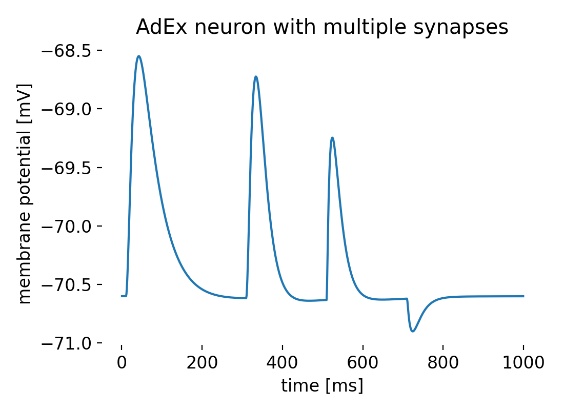
Membrane potential of an AdEx neuron modelled with multiple synapses and synaptic dynamics.

The different synaptic inputs result in distinct effects on the membrane potential of the AdEx neuron. The first synaptic input occurs at approximately 10 ms. This input causes a rapid depolarization of the membrane potential, peaking at around -68.5 mV. Following this peak, the membrane potential decays back towards the resting potential due to the synaptic decay time and adaptation mechanisms. The second synaptic input occurs at 300 ms. Similar to the first input, this causes another depolarization, peaking at approximately the same level (-68.5 mV), followed by a decay back towards the resting potential. The third synaptic input occurs at 500 ms. This input causes another depolarization with characteristics similar to the previous inputs. The fourth synaptic input occurs at 700 ms. Unlike the previous inputs, this one causes a hyperpolarization, creating a trough in the membrane potential around -70.8 mV. Overall, between the synaptic inputs, the membrane potential shows a decay back towards the resting potential, which is around -70.5 mV. The subthreshold and spike-triggered adaptation mechanisms help modulate the membrane potential’s return to the resting state after each depolarization event.

Conclusion

The Exponential Integrate-and-Fire (EIF) and Adaptive Exponential Integrate-and-Fire (AdEx) models provide powerful tools for studying neuronal dynamics. By simplifying the complex Hodgkin-Huxley model, these models capture essential features of neuronal behavior, such as the sharp onset of action potentials and spike-frequency adaptation, while remaining computationally efficient for large-scale simulations. Understanding and applying these models is crucial for advancing our knowledge in computational neuroscience and developing practical applications in neural engineering.

The complete code used in this blog post is available in this Github repositoryꜛ (aeif_neuron.py and aeif_neuron_multple_rices_and_decays.py). Feel free to modify and expand upon it, and share your insights.

References and useful links

• Nicolas Fourcaud-Trocmé, David Hansel, Carl Van Vreeswijk, Nicolas Brunel, How Spike Generation Mechanisms Determine the Neuronal Response to Fluctuating Inputs, 2003, The Journal of Neuroscience, 23(37), 11628–11640, doi: 10.1523/JNEUROSCI.23-37-11628.2003ꜛ
• Wulfram Gerstner, Werner M. Kistler, Richard Naud, and Liam Paninski, Chapter 5 Nonlinear Integrate-and-Fire Models and Chapter 6 Adaptation and Firing Patterns in Neuronal Dynamics: From Single Neurons to Networks and Models of Cognition, 2014, Cambridge University Press, ISBN: 978-1-107-06083-8, Online-Versionꜛ
• Romain Brette and Wulfram Gerstner, Adaptive Exponential Integrate-and-Fire Model as an Effective Description of Neuronal Activity, 2005, Journal of Neurophysiology, 94(5), 3637–3642, doi: 10.1152/jn.00686.2005ꜛ
• Wulfram Gerstner and Romain Brette, Adaptive exponential integrate-and-fire model, 2009, Scholarpedia, 4(6):8427, doi: 10.4249/scholarpedia.8427ꜛ
• Wikipedia article on the EIF and AdEx modelsꜛ
• NEST’s tutorial “Testing the adapting exponential integrate and fire model in NEST (Brette and Gerstner Fig 2C)”ꜛ
• NEST implementation of the AdEx modelꜛ
• NEST’s tutorial “Example of an AEIF neuron with multiple synaptic rise and decay time constants”ꜛ
• NEST’s aeif_cond_alpha model descriptionꜛ
• NEST’s aeif_cond_beta_multisynapse model descriptionꜛ