Example of a neuron driven by an inhibitory and excitatory neuron population

July 28, 2024 6 minute read comments

In this tutorial, we recap the NEST tutorial “Balanced neuron example”ꜛ. We will simulate a neuron driven by an inhibitory and excitatory population of neurons firing Poisson spike trains. The goal is to find the optimal rate for the inhibitory population that will drive the neuron to fire at the same rate as the excitatory population. This short tutorial is quite interesting as it is a practical demonstration of using the NEST simulator to model complex neuronal dynamics.

jpg

Simulation code

We will use the code provided in the NEST tutorial “Balanced neuron example”ꜛ and apply only minor modifications.

First, we need to import the necessary libraries and set the simulation parameters. We will also import the bisect functionꜛ from the scipy package which will help us find the optimal rate for the inhibitory population:

import matplotlib.pyplot as plt
import numpy as np
import nest
import nest.voltage_trace
from scipy.optimize import bisect

nest.set_verbosity("M_WARNING")
nest.ResetKernel()

t_sim = 25000.0  # simulation time [ms]
n_ex = 16000  # size of the excitatory population
n_in = 4000   # size of the inhibitory population
r_ex = 5.0    # mean rate of the excitatory population
r_in = 20.5   # initial rate of the inhibitory population
epsc = 45.0   # peak amplitude of excitatory synaptic currents
ipsc = -45.0  # peak amplitude of inhibitory synaptic currents
d = 1.0       # synaptic delay

We set the firing rate of the excitatory population to 5 Hz and we want to match the firing rate of the neuron to this rate. To do so, we need to find the optimal firing rate for the inhibitory population, which is initially set to 20.5 Hz.

To proceed, we first create the nodes for the neuron and the noise generator (as current input), and a voltmeter, spike recorder, and multimeter for recording the outputs generated by our simulation:

# create nodes:
neuron    = nest.Create("iaf_psc_alpha") # single neuron with alpha-shaped postsynaptic currents
noise     = nest.Create("poisson_generator", 2) # two Poisson generators for the excitatory and inhibitory populations
voltmeter     = nest.Create("voltmeter")
spikerecorder = nest.Create("spike_recorder")
multimeter    = nest.Create("multimeter")
multimeter.set(record_from=["V_m"]) # record the membrane potential of the neuron to which the multimeter will be connected

# define the noise rates for the excitatory and inhibitory populations:
noise.rate = [n_ex * r_ex, n_in * r_in]

Nest, we connect the nodes,

nest.Connect(neuron, spikerecorder)
nest.Connect(multimeter, neuron)
nest.Connect(voltmeter, neuron)
nest.Connect(noise, neuron, syn_spec={"weight": [[epsc, ipsc]], "delay": 1.0})

and run the simulation:

lower = 15.0  # lower bound of the search interval using bisect
upper = 25.0  # upper bound of the search interval using bisect
prec = 0.01   # precision of the bisect search

def output_rate(guess):
    print("Inhibitory rate estimate: %5.2f Hz" % guess)
    rate = float(abs(n_in * guess))
    noise[1].rate = rate # update the Poisson firing rate of the inhibitory population
    spikerecorder.n_events = 0
    nest.Simulate(t_sim)
    out = spikerecorder.n_events * 1000.0 / t_sim
    print(f"  -> Neuron rate: {out} Hz (goal: {r_ex} Hz)")
    return out

in_rate = bisect(lambda x: output_rate(x) - r_ex, lower, upper, xtol=prec)
print(f"Optimal rate for the inhibitory population: {in_rate} Hz")

Note, that the defined function output_rate is used to estimate and update the firing rate of the inhibitory population. The function takes the firing rate of the inhibitory neurons as an argument. It scales the rate with the size of the inhibitory population and configures the inhibitory Poisson generator (noise[1]) accordingly. Then, the spike counter of the spike_recorder is reset to zero and the network is simulated. The return value out is the firing rate of the target neuron in Hz.

output_rate is called within the bisect function. In general, bisectꜛ is a root-finding algorithm for a given function and interval. bisect receives four arguments. First a function is passed whose zero crossing is to be determined. Here, the firing rate of the target neuron should equal the firing rate of the neurons of the excitatory population. Thus we define an anonymous function (using Python’s lambda function) that returns the difference between the actual rate of the target neuron (output_rate(x)) and the rate of the excitatory Poisson generator (r_ex). The lower and upper bound of the interval define the search interval for the zero crossing. The fourth argument is the desired relative precision of the zero crossing (here: 0.01).

bisect loops through the search interval and calls output_rate with the current guess for the inhibitory rate and returns the current firing rate of the target neuron. If the firing rate of the target neuron is close enough to the desired rate of the excitatory population, the zero crossing is found and the optimal rate for the inhibitory population is then printed:

Inhibitory rate estimate: 15.00 Hz
  -> Neuron rate: 347.56 Hz (goal: 5.00 Hz)
Inhibitory rate estimate: 25.00 Hz
  -> Neuron rate:   0.04 Hz (goal: 5.00 Hz)
Inhibitory rate estimate: 20.00 Hz
  -> Neuron rate:  35.80 Hz (goal: 5.00 Hz)
Inhibitory rate estimate: 22.50 Hz
  -> Neuron rate:   0.00 Hz (goal: 5.00 Hz)
Inhibitory rate estimate: 21.25 Hz
  -> Neuron rate:   0.80 Hz (goal: 5.00 Hz)
Inhibitory rate estimate: 20.62 Hz
  -> Neuron rate:   8.52 Hz (goal: 5.00 Hz)
Inhibitory rate estimate: 20.94 Hz
  -> Neuron rate:   3.24 Hz (goal: 5.00 Hz)
Inhibitory rate estimate: 20.78 Hz
  -> Neuron rate:   4.96 Hz (goal: 5.00 Hz)
Inhibitory rate estimate: 20.70 Hz
  -> Neuron rate:   6.52 Hz (goal: 5.00 Hz)
Inhibitory rate estimate: 20.74 Hz
  -> Neuron rate:   5.76 Hz (goal: 5.00 Hz)
Inhibitory rate estimate: 20.76 Hz
  -> Neuron rate:   5.12 Hz (goal: 5.00 Hz)
Inhibitory rate estimate: 20.77 Hz
  -> Neuron rate:   5.20 Hz (goal: 5.00 Hz)
Optimal rate for the inhibitory population: 20.77 Hz

The optimal rate for the inhibitory population is 20.77 Hz.

As a last step, we extract the recorded data from the multimeter and plot corresponding membrane potential of the neuron:

# extract recorded data from the multimeter and plot it:
recorded_events = multimeter.get()
recorded_V = recorded_events["events"]["V_m"]
time = recorded_events["events"]["times"]
spikes = spikerecorder.get("events")
senders = spikes["senders"]

plt.figure(figsize=(7, 5))
plt.plot(time, recorded_V, label="membrane potential")
plt.xlabel("time (ms)")
plt.ylabel("membrane potential (mV)")
plt.title(f"Membrane potential of a {neuron.get('model')} neuron")
plt.gca().spines["top"].set_visible(False)
plt.gca().spines["bottom"].set_visible(False)
plt.gca().spines["left"].set_visible(False)
plt.gca().spines["right"].set_visible(False)
plt.legend(loc="lower left")
plt.tight_layout()
plt.show()

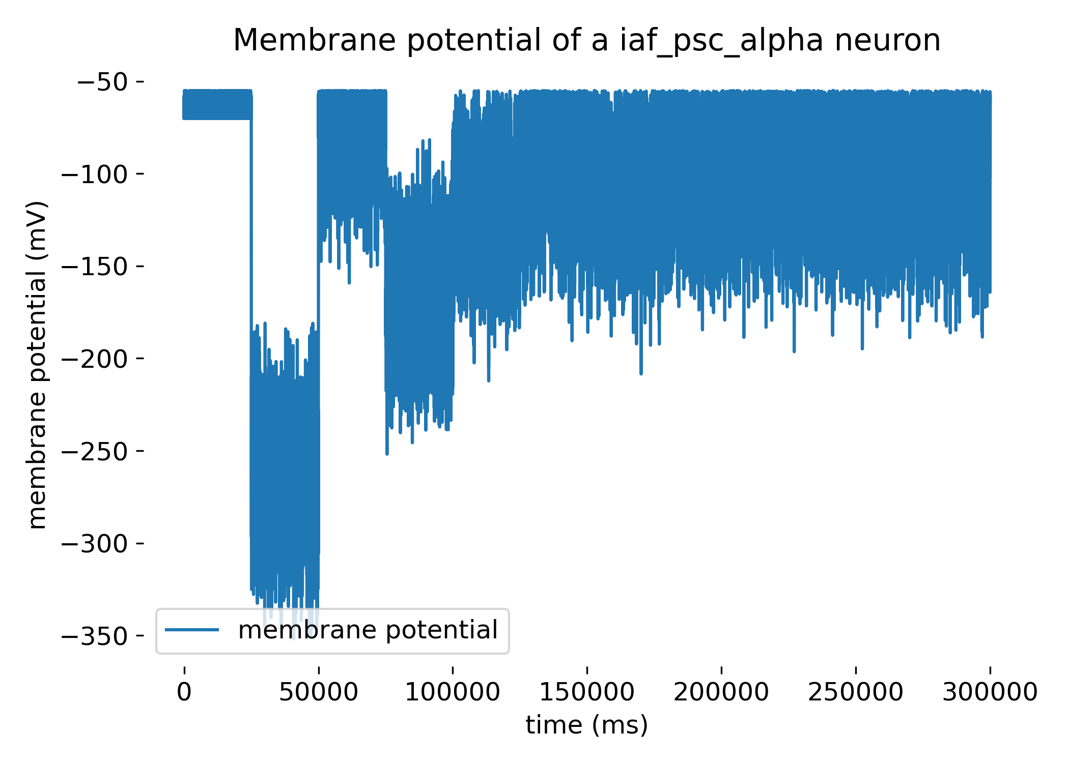
Membrane potential of a iaf_psc_alpha neuron. The membrane potential of the neuron is driven by an excitatory and inhibitory population of neurons. We found an optimal rate for the inhibitory population (20.77 Hz) that drives the neuron to fire at the same rate as the excitatory population (5 Hz).

The plot represents the membrane potential of the modelled iaf_psc_alpha neuron over a simulated time of 300,000 ms receiving excitatory and inhibitory inputs. The membrane potential fluctuates between about -50 mV and roughly -350 mV. These fluctuations are primarily driven by the balance of excitatory and inhibitory synaptic inputs modeled through Poisson spike trains. Sharp drops in membrane potential (hyperpolarizations) can be observed, followed by gradual recoveries (depolarizations). These are indicative of the neuron receiving strong inhibitory inputs followed by periods of reduced input, allowing the membrane potential to return towards a baseline. There are periods where the membrane potential appears relatively stable, especially noticeable around 0 to 25,000 ms and around 100,000 ms until nearing 300,000 ms. During these phases, the balance between inhibitory and excitatory inputs likely reaches a temporary equilibrium.

Conclusion

NEST is very versatile and can be used to study the responses of single neurons or complex neural networks. In the presented NEST tutorial “Balanced neuron example”ꜛ, we simulated a neuron driven by an inhibitory and excitatory population of neurons firing Poisson spike trains. By applying an iterative approach, we found the optimal rate for the inhibitory population that drives the single neuron to fire at the same rate as the excitatory population.

The iterative adjustment process demonstrates the precision NEST offers for neural simulations. This method provides valuable insights into neuronal behavior and can be extended to more complex models and networks.

The modified code used in this blog post is available in this Github repositoryꜛ (neuron_with_population_inputs.py). Feel free to modify and expand upon it, and share your insights.

References and useful links

NEST tutorial “Balanced neuron example”ꜛ
Jochen Martin Eppler, Moritz Helias, Eilif Muller, Markus Diesmann, Marc-Oliver Gewaltig, PyNEST: A convenient interface to the NEST simulator, 2009, Front. Neuroinform, DOI: 10.3389/neuro.11.012.2008ꜛ