Brunel network: A comprehensive framework for studying neural network dynamics

In his work from 2000ꜛ, Nicolas Brunel introduced a comprehensive framework for studying the dynamics of sparsely connected networks. The network is based on spiking neurons with random connectivity and differently balanced excitation and inhibition. It is characterized by a high level of sparseness and a low level of firing rates. The model is able to reproduce a wide range of neural dynamics, including both synchronized regular and asynchronous irregular activity as well as global oscillations. In this post, we summarize the essential concepts of that network and replicate the main results using the NEST simulator.

Model description

Brunel’s model focuses on large networks of leaky integrate-and-fire (LIF) neurons divided into $N_{ex}$ excitatory and $N_{in}$ inhibitory populations. The network is characterized by sparse connectivity, where each neuron connects to a small, random subset of other neurons. The membrane potential $V_i(t)$ of neuron $i$ evolves according to:

\[\tau_m \frac{dV_i(t)}{dt} = -V_i(t) + R I_i(t)\]

where

• $\tau_m$ is the membrane time constant,
• $R$ is the membrane resistance, and
• $I_i(t)$ is the total synaptic input current to neuron $i$.

The synaptic input $I_i(t)$ is the sum of the excitatory and inhibitory postsynaptic potentials (PSPs) received from other neurons:

\[I_i(t) = \sum_j J_{ij} \sum_k \delta(t - t_j^k - D)\]

where

• $J_{ij}$ represents the synaptic weight from neuron $j$ to neuron $i$,
• $t_j^k$ are the spike times of neuron $j$,
• $D$ is the synaptic delay, and
• $\delta(t)$ is the Dirac delta function.

Connectivity

The connection probabilities are given by $\epsilon$, which controls the sparseness of the network. The number of excitatory ($C_E$) and inhibitory ($C_I$) synapses per neuron, which define the total number of connections, is determined by:

\[\begin{align*} C_E &= \epsilon N_E \\ C_I &= \epsilon N_I \end{align*}\]

Synaptic weights

Synaptic weights for excitatory ($J$) and inhibitory ($-gJ$) connections are defined, where $g$ is the ratio of inhibitory to excitatory synaptic strength.

External input

Each neuron also receives external input modeled as a Poisson process with rate $\nu_{\text{ext}}$. The external rate is related to the threshold rate $\nu_{\text{th}}$ by:

\[\nu_{\text{ext}} = \eta \nu_{\text{th}}\]

where

• $\eta$ is a scaling factor, and
• $\nu_{\text{th}}$ is the threshold rate, calculated as the rate at which the input alone would drive the neuron to threshold.

Postsynaptic currents

The postsynaptic current resulting from a spike is characterized by an exponential function with a synaptic time constant $\tau_{\text{syn}}$:

\[I(t) = J e^{\left(-\frac{t}{\tau_{\text{syn}}}\right)}\]

Mean-field approximation and Fokker-Planck equation

A common approach to analyzing large networks is to use a mean-field approximation, which replaces the individual neurons with population averages. This simplifies the network dynamics and allows for analytical solutions. The dynamics of the network can then be described using a Fokker-Planck equation for the probability distribution $P(V, t)$ of the membrane potential $V$:

\[\begin{align*} \tau \frac{\partial P(V, t)}{\partial t} =& \frac{\sigma^2(t)}{2} \frac{\partial^2 P(V, t)}{\partial V^2} \\ &+ \frac{\partial}{\partial V} [(V - \mu(t)) P(V, t)] \end{align*}\]

where $\mu(t)$ and $\sigma(t)$ are the mean and standard deviation of the input current, respectively:

\[\begin{align*} \mu &= \tau_m \nu (C_E J - C_I gJ) \\ \sigma^2 &= \tau_m \nu (C_E J^2 + C_I (gJ)^2) \end{align*}\]

The firing rate $\nu(t)$ is given by the probability current at the membrane threshold potential $\theta$:

\[\nu(t) = -\frac{\sigma^2(t)}{2\tau} \left. \frac{\partial P(V, t)}{\partial V} \right|_{V=\theta}\]

Threshold rate

The threshold rate $\nu_{\text{th}}$, required to drive the network to a stable firing rate, is calculated as:

\[\nu_{\text{th}} = \frac{\theta C_m}{J_{\text{ex}} C_E \exp(1) \tau_m \tau_{\text{syn}}}\]

where

• $\theta$ is the membrane threshold potential,
• $C_m$ is the membrane capacitance,
• $J_{\text{ex}}$ is the normalized excitatory postsynaptic potential (PSP) amplitude, abd
• $\exp(1)$ is the base of the natural logarithm.

The external rate $\nu_{\text{ext}}$ is then:

\[\nu_{\text{ext}} = \eta \nu_{\text{th}}\]

Key factors controlling network dynamics

In summary, the following factors control the overall dynamics of the network:

• synaptic weight ratio $g$: The factor $g$ represents the ratio of inhibitory to excitatory synaptic strength. It determines how inhibitory synaptic inputs balance the excitatory inputs in the network.
• external input rate $\nu_{\text{ext}}$: The rate of the Poisson process providing external input to each neuron is a critical factor in maintaining activity within the network.
• threshold rate $\nu_{\text{th}}$: The rate at which a neuron would reach its firing threshold based solely on the input current; this parameter helps in defining the necessary external rate to keep the neurons active.
• scaling factor $\eta$: This factor scales the external input rate $\nu_{\text{ext}}$ relative to the threshold rate $\nu_{\text{th}}$. It determines the intensity of external stimulation necessary to maintain desired network dynamics, influencing the overall activity level of the network.
• synaptic time constant $\tau_{\text{syn}}$: The time constant of the postsynaptic current determines the decay rate of the synaptic input following a spike, influencing the temporal integration of synaptic inputs.
• synaptic delay $D$: The delay in synaptic transmission affects the temporal relationship between spikes in the network, influencing the synchronization and propagation of activity.

Depending on the balance of these factors, the network can exhibit a wide range of dynamics, from asynchronous irregular activity to synchronized oscillations:

• synchronous regular (SR) activity: neurons are almost fully synchronized and behave as oscillators when excitation dominates inhibition and synaptic time distributions are sharply peaked
• asynchronous regular (AR) activity: stationary global activity and quasi-regular individual neuron firing when excitation dominates inhibition and synaptic time distributions are broadly peaked;
• asynchronous irregular (AI) activity: stationary global activity but strongly irregular individual firing at low rates when inhibition dominates excitation in an intermediate range of external frequencies;
• synchronous irregular (SI) activity: oscillatory global activity but strongly irregular individual firing at low (compared to the global oscillation frequency) firing rates, when inhibition dominates excitation and either low external frequencies (slow oscillations) or high external frequencies (fast oscillations).

For instance, depending on the choice of the synaptic delay $D$, the regimes of these four activity states in dependence of the choice of synaptic weights ratio $g$ and the ratio of external input rate $\nu_{\text{ext}}$ to threshold rate $\nu_{\text{th}}$ (thus, $\eta$) can vary significantly, as can be seen in the phase diagrams in figure 2 of Brunel (2000)ꜛ.

In the Python simulation code below, we will set the postsynaptic amplitude $J$ to 0.1 mV and the synaptic delay $D$ to 1.5 ms. The corresponding phase diagram looks in accordance to the one presented in figure 7 of Brunel (2000)ꜛ:

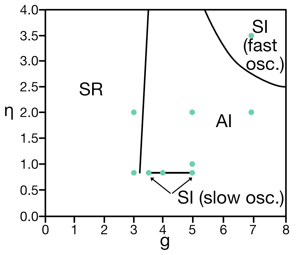
Sketch reproducing figure 7 from Brunel (2000)ꜛ: Phase diagram of the network dynamics in the $g-\eta$ plane for $D$ = 1.5 ms, $J$ = 0.1 mV, $C_E$ = 1000, $C_I$ = 250, $\epsilon$ = 0.1. Indicated are the four different network states: asynchronous irregular (AI), synchronous irregular (SI), asynchronous regular (AR), and synchronous regular (SR). The black lines represent the boundaries between the different states. Green dots indicate the parameter values used in the simulation below.

Python simulation

We will adapt and slightly modify the original code from the NEST tutorial “Random balanced network (alpha synapses) connected with NEST”ꜛ. To replicate the results from Figure 8 in Brunel (2000)ꜛ, we will simulate $N_{\text{ex}} = 10000$ excitatory neurons along with $N_{\text{in}} = 250$ inhibitory neurons. The synaptic delay $D$ and the synaptic time constant $\tau_{\text{syn}}$ are set to 1.5 ms and 0.5 ms, respectively. The connection probability $\epsilon$ is set to 0.1, and the number of connections, $C_E$ and $C_I$, is set to 1000 and 250, respectively. The synaptic weights $J$ is set to 0.1 mV, the membrane time constant $\tau_m$ is set to 20 ms, and the membrane capacitance $C_m$ is set to 250 pF. The membrane threshold potential $\theta$ is set to 20 mV. The simulation will run for 1000 ms with a resolution of 0.1 ms. We will run the simulation for various values of the synaptic weights ratio $g$ and the ratio $\eta$ of the external input rate $\nu_{\text{ext}}$ and the threshold rate $\nu_{\text{th}}$ to observe the different network states. Note that for visualization purposes, we record spike events from only 50 excitatory neurons (it is not necessary to track all 10,000 excitatory neurons).

Let’s begin by importing the necessary libraries and defining two helper-functions to compute the maximum of the postsynaptic potential (PSP) for a current of unit amplitude and the Lambert W functionꜛ for $x < 0$:

import matplotlib.pyplot as plt
import matplotlib.gridspec as gridspec
import numpy as np
import nest
import scipy.special as sp

# set global properties for all plots:
plt.rcParams.update({'font.size': 12})
plt.rcParams["axes.spines.top"]    = False
plt.rcParams["axes.spines.bottom"] = False
plt.rcParams["axes.spines.left"]   = False
plt.rcParams["axes.spines.right"]  = False

def LambertWm1(x):
    """ 
    Here we define the Lambert W function for x < 0. The function is usually used
    in the context of the Brunel network to compute the maximum of the PSP (postsynaptic
    potential) for a current of unit amplitude.     
    """
    # using scipy to mimic the gsl_sf_lambert_Wm1 function:
    return sp.lambertw(x, k=-1 if x < 0 else 0).real

def ComputePSPnorm(tauMem, CMem, tauSyn):
    """ 
    This function computes the maximum of the PSP for a current of unit amplitude.
    """
    a = tauMem / tauSyn
    b = 1.0 / tauSyn - 1.0 / tauMem

    # time of maximum
    t_max = 1.0 / b * (-LambertWm1(-np.exp(-1.0 / a) / a) - 1.0 / a)

    # maximum of PSP for current of unit amplitude:
    return (
        np.exp(1.0)
        / (tauSyn * CMem * b)
        * ((np.exp(-t_max / tauMem) - np.exp(-t_max / tauSyn)) / b - t_max * np.exp(-t_max / tauSyn))
    )

Next, we define the parameters of the network and set up the simulation:

# set the simulation resolution and time:
dt = 0.1          # the resolution in ms
simtime = 1000.0  # Simulation time in ms
delay = 1.5         # synaptic delay in ms; also controls the dynamics of the network

nest.set_verbosity("M_WARNING")
nest.ResetKernel()
nest.resolution = dt
nest.print_time = False
nest.overwrite_files = True

# set the parameters of the network:
g = 3.5          # ratio inhibitory weight/excitatory weight
eta = 0.9        # defines the ration between external rate and threshold rate
epsilon = 0.1    # connection probability

order = 2500    # scaling factor for number of neurons
NE = 4 * order  # number of excitatory neurons
NI = 1 * order  # number of inhibitory neurons
N_neurons = NE + NI  # number of neurons in total
N_rec = 50      # record from 50 neurons instead of all (for visualization in the plots later
                # and similar to Brunel's original publication)

CE = int(epsilon * NE)  # number of excitatory synapses per neuron
CI = int(epsilon * NI)  # number of inhibitory synapses per neuron
C_tot = int(CI + CE)    # total number of synapses per neuron

tauSyn = 0.5  # synaptic time constant in ms
tauMem = 20.0 # time constant of membrane potential in ms
CMem = 250.0  # capacitance of membrane in in pF
theta = 20.0  # membrane threshold potential in mV
neuron_params = {
    "C_m": CMem,
    "tau_m": tauMem,
    "tau_syn_ex": tauSyn,
    "tau_syn_in": tauSyn,
    "t_ref": 2.0,
    "E_L": 0.0,
    "V_reset": 0.0,
    "V_m": 0.0,
    "V_th": theta}
J = 0.1  # postsynaptic amplitude in mV
J_unit = ComputePSPnorm(tauMem, CMem, tauSyn)
J_ex = J / J_unit # amplitude of excitatory postsynaptic current
J_in = -g * J_ex  # amplitude of inhibitory postsynaptic current

# define the threshold rate, which is the external rate needed to fix the membrane 
# potential around its threshold, as well as the external firing rate and the rate 
# of the poisson generator which is multiplied by the in-degree CE and converted to 
# Hz by multiplication by 1000:
nu_th = (theta * CMem) / (J_ex * CE * np.exp(1) * tauMem * tauSyn) # threshold rate
nu_ex = eta * nu_th # external rate
p_rate = 1000.0 * nu_ex * CE # rate of the Poisson generator

Now, we create the nodes and establish connections between them:

# create the nodes:
nodes_ex = nest.Create("iaf_psc_alpha", NE, params=neuron_params)
nodes_in = nest.Create("iaf_psc_alpha", NI, params=neuron_params)
noise    = nest.Create("poisson_generator", params={"rate": p_rate})
exspikes = nest.Create("spike_recorder") # record excitatory spikes
inspikes = nest.Create("spike_recorder") # record inhibitory spikes

exspikes.set(label="brunel-py-ex", record_to="memory")
inspikes.set(label="brunel-py-in", record_to="ascii") # record to ascii=to file (for memory reasons)

# make the connections:
# create a copy of the static_synapse model and set its default the weight and delay parameters:
nest.CopyModel("static_synapse", "excitatory", {"weight": J_ex, "delay": delay})
nest.CopyModel("static_synapse", "inhibitory", {"weight": J_in, "delay": delay})

# connect the noise to the excitatory and inhibitory nodes  (using default all-to-all rule):
nest.Connect(noise, nodes_ex, syn_spec="excitatory")
nest.Connect(noise, nodes_in, syn_spec="excitatory")

# connect the spike recorders to the excitatory and inhibitory nodes:
nest.Connect(nodes_ex[:N_rec], exspikes, syn_spec="excitatory")
nest.Connect(nodes_in[:N_rec], inspikes, syn_spec="excitatory")

# connect the excitatory nodes:
conn_params_ex = {"rule": "fixed_indegree", "indegree": CE}
nest.Connect(nodes_ex, nodes_ex + nodes_in, conn_params_ex, "excitatory")

# connect the inhibitory nodes:
conn_params_in = {"rule": "fixed_indegree", "indegree": CI}
nest.Connect(nodes_in, nodes_ex + nodes_in, conn_params_in, "inhibitory")

Finally, we simulate the network (depending on your machine and the chosen setting, this can take a while):

nest.Simulate(simtime)

When the simulation run is completed, we can extract the number of events and the firing rate:

# extract the number of events and the firing rate:
events_ex = exspikes.n_events
events_in = inspikes.n_events

rate_ex = events_ex / simtime * 1000.0 / N_rec
rate_in = events_in / simtime * 1000.0 / N_rec

num_synapses_ex = nest.GetDefaults("excitatory")["num_connections"]
num_synapses_in = nest.GetDefaults("inhibitory")["num_connections"]
num_synapses = num_synapses_ex + num_synapses_in

# print some information about the simulation:
print("Brunel network simulation (Python)")
print(f"Number of neurons : {N_neurons}")
print(f"Number of synapses: {num_synapses}")
print(f"       Excitatory : {num_synapses_ex}")
print(f"       Inhibitory : {num_synapses_in}")
print(f"Excitatory rate   : {rate_ex:.2f} Hz")
print(f"Inhibitory rate   : {rate_in:.2f} Hz")

For plotting, we extract the spike times and neuron IDs from the excitatory spike recorder and pipe them into a scatter plot and a histogram of the spiking rate:

# extract the spike times and neuron IDs from the excitatory spike recorder:
spike_events = nest.GetStatus(exspikes, "events")[0]
spike_times = spike_events["times"]
neuron_ids = spike_events["senders"]

# combine the spike times and neuron IDs into a single array and sort by time:
spike_data = np.vstack((spike_times, neuron_ids)).T
spike_data_sorted = spike_data[spike_data[:, 0].argsort()]

# extract sorted spike times and neuron IDs:
sorted_spike_times = spike_data_sorted[:, 0]
sorted_neuron_ids = spike_data_sorted[:, 1]

# spike raster plot and histogram of spiking rate:
fig = plt.figure(figsize=(6, 6))
gs = gridspec.GridSpec(5, 1)

ax1 = plt.subplot(gs[0:4, :])
ax1.scatter(sorted_spike_times, sorted_neuron_ids, s=9.0, color='mediumaquamarine', alpha=1.0)
plt.title(f"50 example excitatory neurons (out of {NE})\ng: {g}, $\\nu_/\\nu_$: {nu_ex/nu_th}, delay: {delay}, $\eta$: {eta}, $\epsilon$: {epsilon}")
#ax1.set_xlabel("time [ms]")
ax1.set_xticks([])
ax1.set_ylabel("neuron ID")
ax1.set_xlim([0, simtime+5])
ax1.set_ylim([0, N_rec+1])
ax1.set_yticks(np.arange(0, N_rec+1, 10))

ax2 = plt.subplot(gs[4, :])
hist_binwidth = 5.0
t_bins = np.arange(np.amin(sorted_spike_times), np.amax(sorted_spike_times), hist_binwidth)
n, bins = np.histogram(sorted_spike_times, bins=t_bins)
heights = 1000 * n / (hist_binwidth * (N_rec))
ax2.bar(t_bins[:-1], heights, width=hist_binwidth, color='violet')
#ax2.set_title(f"histogram of spiking rate vs. time")
ax2.set_ylabel("firing rate\n[Hz]")
ax2.set_xlabel("time [ms]")
ax2.set_xlim([0, simtime+5])
ax2.set_ylim([0, 200])

plt.tight_layout()
plt.show()

Results

I wasn’t able to reproduce Brunel’s results exactly, but the network dynamics are consistent with the expected behavior. The $g$ and $\eta$ value pairs to not exactly match the ones in the original publication, but the network states are still clearly distinguishable. Reasons for the discrepancy could be the different random number generator seeds used in the simulation or the different number of recorded neurons. In the following, I will therefore present the results of “my own” little parameter study.

Synchronized network activity with global irregular oscillations (SI)

Fixing $\eta$ to 0.9 and varying $g$ from 3.5 to 4.0, we observe the following network states:

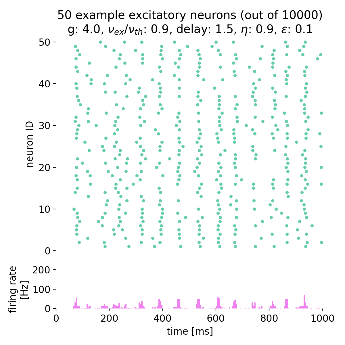
Spike raster plots (top) and histograms of the spiking rate (bottom) for $g = 3.5$ (left) and $g = 4.0$ (right) with $\eta = 0.9$.

The neurons fire synchronously. The histograms show the firing rate of the network over time, with global oscillatory behavior clearly visible. However, the frequency of the oscillations is not constant, but irregular. The firing rate is higher for $g = 3.5$ compared to $g = 4.0$, reflecting the stronger inhibitory influence in the latter case. This indicates that the network is in the (slow) synchronous irregular (SI) activity state.

Asynchronous network activity with irregular global firing (AI)

As soon as we further increase $g$ to, e.g., 5.0, the network transitions to asynchronous irregular activity, i.e., the neurons are not synchronized anymore, with stationary global activity (no oscillations) and individual firing at low rates. The network dynamics are no longer synchronized, and the firing rate is significantly lower compared to the synchronized state:

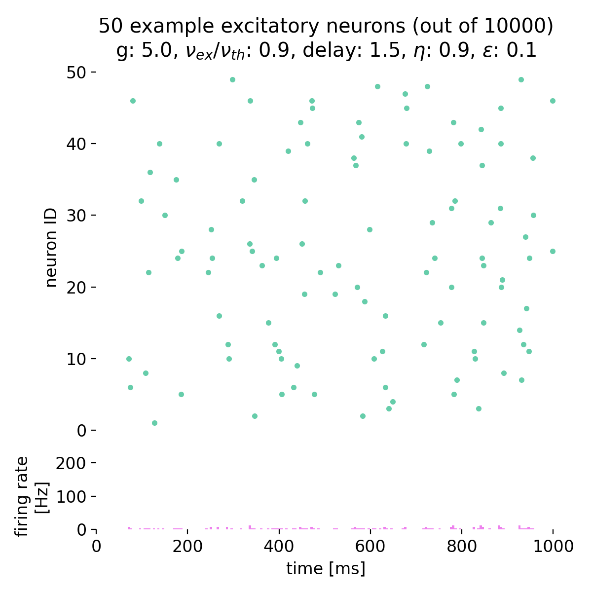
Spike raster plots (top) and histograms of the spiking rate (bottom) for $g = 5.0$ and $\eta = 0.9$. The network transitions into the state of asynchronous irregular (AI) activity.

The network transitioned into the state of asynchronous irregular (AI) activity.

Increasing both, $g$ and $\eta$, will keep the network in this asynchronous state, but with varying firing rates:

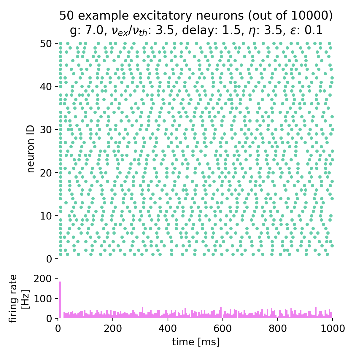
Spike raster plots and histograms of the spiking rate for $g = 5.0$ and $\eta = 1.0$ (top left), $g = 5.0$ and $\eta = 2.0$ (top right), $g = 7.0$ and $\eta = 2.0$ (bottom left), and $g = 7.0$ and $\eta = 3.5$ (bottom right). The network is in the asynchronous irregular (AI) activity state.

Surprisingly, the simulation with $g = 7.0$ and $\eta = 3.5$ still shows the network in the asynchronous irregular (AI) activity state, while the phase diagram in figure 7 of Brunel (2000)ꜛ (or see phase diagram sketch above) suggests that the network should be in the synchronous irregular (SI) activity state with fast oscillations. This discrepancy could be due to the different frameworks used for the simulation, different random number generator seeds or other factors.

Fully synchronized network activity with constant global firing (SR)

Setting $g$ to 3.0 and varying $\eta$ from 0.9 to 2.0, we observe that the neurons fire synchronously at high rates, but no global oscillations are present, just a constant high firing rate. The network is in the synchronous regular (SR) activity state:

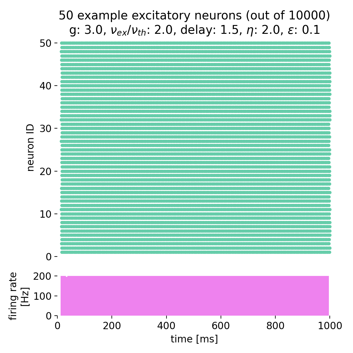
Spike raster plots and histograms of the spiking rate for $g = 3.0$ and $\eta = 0.9$ (left) and $g = 3.0$ and $\eta = 2.0$ (right). The network is in the synchronous regular (SR) activity state.

Conclusion

The Brunel network model provides a robust framework for studying the dynamics of neural networks with excitatory and inhibitory neurons. By examining the balance of these inputs, the model reveals insights into network states, synchronization, and neural coding. The mathematical foundation and simulation code illustrate the complex interactions within the network, offering valuable tools for computational neuroscience research. The NEST simulator provides a powerful platform for implementing and analyzing such models, enabling us to explore the dynamics of large-scale neural networks.

The complete code used in this blog post is available in this Github repositoryꜛ (brunel_network.py). Feel free to modify and expand upon it, and share your insights.

References and useful links

• Nicolas Brunel, Dynamics of Sparsely Connected Networks of Excitatory and Inhibitory Spiking Neurons, 2000, Journal of Computational Neuroscience, 8(3), 183–208, doi: 10.1023/A:1008925309027ꜛ
• Wulfram Gerstner, Werner M. Kistler, Richard Naud, and Liam Paninski, Chapter 13 Continuity Equation and the Fokker-Planck Approach in Neuronal Dynamics: From Single Neurons to Networks and Models of Cognition, 2014, Cambridge University Press, ISBN: 978-1-107-06083-8, free online versionꜛ
• M.O. Gewaltig, A. Morrison, H. E. Plesser, NEST by Example: An Introduction to the Neural Simulation Tool NEST in Computational Systems Neurobiology, 2012, Springer, Dordrecht, doi: 10.1007/978-94-007-3858-4_18ꜛ (free eBook)
• NEST’s tutorial “Random balanced network (alpha synapses) connected with NEST”ꜛ
• NEST’s iaf_psc_alpha model descriptionꜛ
• NEST’s iaf_psc_alpha implementationꜛ