Izhikevich SNN simulated with NEST

June 30, 2024 11 minute read comments

In this post, we explore how easy it is it is to set up a large-scale, multi-population spiking neural network (SNN) with the NEST simulator. We simulate a simple SNN comprising two distinct populations of Izhikevich neurons, demonstrating the efficiency and flexibility of NEST and its capability to handle complex neural network simulations with ease.

jpg Example of a two-population SNN simulation consisting of 200 chattering and 800 regular spiking Izhikevich neurons.

For a basic introduction into NEST, please refer to the previous post.

Setting up populations of neurons in NEST

Before we start with the simulation, we will first take a general look at how to set up populations of neurons in NEST.

Creating parameterized populations of neurons

NEST’s nest.Create()ꜛ function receives four arguments: the model name, the number of neurons to create (default: 1), a dictionary of parameters (optional), and a list of positions (optional):

nest.Create(model, n=1, params=None, positions=None)

The model can be any model supported by NESTꜛ. The params dictionary contains the parameters of the neurons to be created, which depend on the chosen model. If no parameters are provided, NEST will use the default parameters of the selected model. With the positions argument, spatial positions of the neurons can be defined. If no positions are provided, the neurons have no spatial attachment.

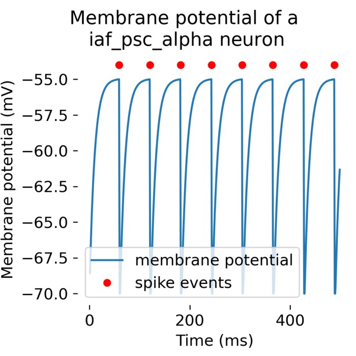
Let’s take a look at some examples. We first create a population of 100 iaf_psc_alphaꜛ neurons with a constant external input current of 200 pA and a membrane time constant of 20 ms. The parameters are provided as a dictionary:

ndict = {"I_e": 200.0, "tau_m": 20.0}
neuronpop = nest.Create("iaf_psc_alpha", 100, params=ndict)

A list of all parameters of a specific model can be obtained using the nest.GetDefaults()ꜛ function:

nest.GetDefaults(neuronpop.model)

Custom model parameter values can also be set before creating the population of neurons, which allows for simulations being more flexible. To do so, we make use of the nest.SetDefaults()ꜛ function:

ndict = {"I_e": 200.0, "tau_m": 20.0}
nest.SetDefaults("iaf_psc_alpha", ndict)
neuronpop1 = nest.Create("iaf_psc_alpha", 100)
neuronpop2 = nest.Create("iaf_psc_alpha", 100)
neuronpop3 = nest.Create("iaf_psc_alpha", 100)

If we want to have a variant of the iaf_psc_alpha model with a different external input current, we can copy the model with nest.CopyModel()ꜛ and set the new parameters accordingly:

edict = {"I_e": 200.0, "tau_m": 20.0}
nest.CopyModel("iaf_psc_alpha", "exc_iaf_psc_alpha")
nest.SetDefaults("exc_iaf_psc_alpha", edict)

or in one step:

idict = {"I_e": 300.0}
nest.CopyModel("iaf_psc_alpha", "inh_iaf_psc_alpha", params=idict)

The new models are added to NEST’s model list (nest.Models()) until you reset the kernel. The copied models can now be used to create different populations of neurons:

epop1 = nest.Create("exc_iaf_psc_alpha", 100)
epop2 = nest.Create("exc_iaf_psc_alpha", 100)
ipop1 = nest.Create("inh_iaf_psc_alpha", 30)
ipop2 = nest.Create("inh_iaf_psc_alpha", 30)

It is also possible to assign individual parameter values to each neuron in a population. To do so, we would provide a list of dictionaries with the parameter values for each neuron. If we want to assign individual values just for some parameters, NEST has no problem to receive an inhomogeneous set of parameters:

parameter_dict = {"I_e": [200.0, 150.0], "tau_m": 20.0, "V_m": [-77.0, -66.0]}
pop3 = nest.Create("iaf_psc_alpha", 2, params=parameter_dict)

print(pop3.get(["I_e", "tau_m", "V_m"]))

The two individual values for I_e as well as for V_m are assigned to the two neurons in the population. The single value for tau_m is applied to both neurons.

Randomizing the parameters of the neurons

In case you need a randomization of the parameters of your neurons, you can use list comprehensions to create a list of random values. For instance, to randomize the membrane potential of a neuron population between -70 mV and -55 mV:

Vth=-55.
Vrest=-70.
dVms =  {"V_m": [Vrest+(Vth-Vrest)*numpy.random.rand() for x in range(len(epop1))]}
epop1.set(dVms)

Alternatively, you can also use NEST’s random parameters and distributions. NEST has a number of such parameters which can be combined and used with some mathematical functions provided by NEST:

epop1.set({"V_m": Vrest + nest.random.uniform(0.0, Vth-Vrest)})

Connecting neuron populations

To connect two populations, we can simply use NEST’s nest.Conncetion() function that we have extensively discussed in the previous post. For instance, to connect the epop1 population to the ipop1 population with a fixed indegree of 10, simply use:

conn_dict_epop_to_ipop = {"rule": "fixed_indegree", "indegree": 10}
nest.Connect(epop1, ipop1, conn_dict_epop_to_ipop)

Similarly, to connect the two populations to a multimeter:

multimeter = nest.Create("multimeter")
multimeter.set(record_from=["V_m"])

nest.Connect(multimeter, epop1)
nest.Connect(multimeter, ipop1)

nest.Connect(epop1 + ipop1, multimeter)

Please read what to consider when connecting multiple neurons to a single recording device.

Setting up the Izhikevich SNN simulation

Now, let’s set up a SNN simulation with two distinct populations of Izhikevich neurons.

First, we reuse the Izhikevich neuron model definitions from the previous example:

import os
import matplotlib.pyplot as plt
import numpy as np
import nest

# set the verbosity of the NEST simulator:
nest.set_verbosity("M_WARNING")

# reset the kernel for safety:
nest.ResetKernel()

# define sets of typical parameters of the Izhikevich neuron model:
p_RS  = [0.02, 0.2, -65, 8, "regular spiking (RS)"] # regular spiking settings for excitatory neurons (RS)
p_IB  = [0.02, 0.2, -55, 4, "intrinsically bursting (IB)"] # intrinsically bursting (IB)
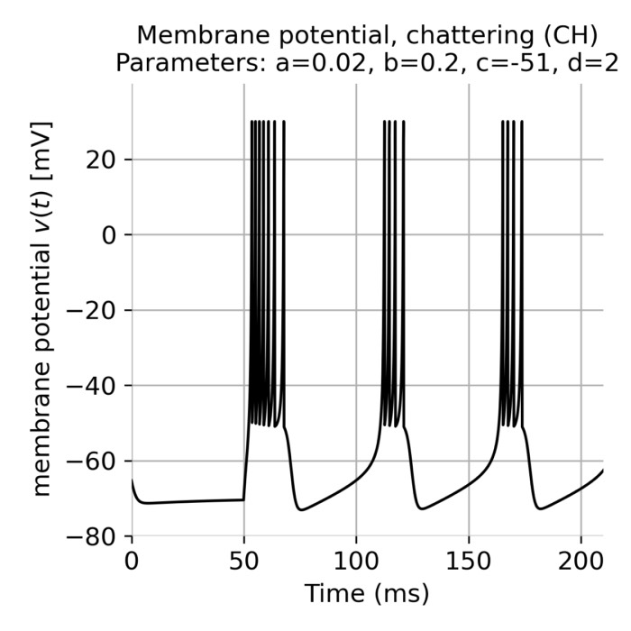
p_CH  = [0.02, 0.2, -51, 2, "chattering (CH)"] # chattering (CH)
p_FS  = [0.1, 0.2, -65, 2, "fast spiking (FS)"] # fast spiking (FS)
p_TC  = [0.02, 0.25, -65, 0.05, "thalamic-cortical (TC)"] # thalamic-cortical (TC) (doesn't work well)
p_LTS = [0.02, 0.25, -65, 2, "low-threshold spiking (LTS)"] # low-threshold spiking (LTS)
p_RZ  = [0.1, 0.26, -65, 2, "resonator (RZ)"] # resonator (RZ)

# copy the Izhikevich neuron model and set the parameters for the different neuron types:
nest.CopyModel("izhikevich", "izhikevich_RS", {"a": p_RS[0], "b": p_RS[1], "c": p_RS[2], "d": p_RS[3]})
nest.CopyModel("izhikevich", "izhikevich_IB", {"a": p_IB[0], "b": p_IB[1], "c": p_IB[2], "d": p_IB[3]})
nest.CopyModel("izhikevich", "izhikevich_CH", {"a": p_CH[0], "b": p_CH[1], "c": p_CH[2], "d": p_CH[3]})
nest.CopyModel("izhikevich", "izhikevich_FS", {"a": p_FS[0], "b": p_FS[1], "c": p_FS[2], "d": p_FS[3]})
nest.CopyModel("izhikevich", "izhikevich_TC", {"a": p_TC[0], "b": p_TC[1], "c": p_TC[2], "d": p_TC[3]})
nest.CopyModel("izhikevich", "izhikevich_LTS", {"a": p_LTS[0], "b": p_LTS[1], "c": p_LTS[2], "d": p_LTS[3]})
nest.CopyModel("izhikevich", "izhikevich_RZ", {"a": p_RZ[0], "b": p_RZ[1], "c": p_RZ[2], "d": p_RZ[3]})

Next, we create two neuron populations consisting of 800 regular spiking (RS) and 200 chattering (CH) Izhikevich neurons. We declare the neuron of the first population as excitatory and the neurons of the second population as inhibitory. We also create a multimeter and a spike recorder to monitor the membrane potential and record the spikes, respectively:

# set up a two-neuron-type network according to Izhikevich's original paper:
Ne = 800  # Number of excitatory neurons
Ni = 200  # Number of inhibitory neurons
T = 1000.0 # Simulation time (ms)
population_e     = nest.Create("izhikevich_RS", n=Ne)
population_i     = nest.Create("izhikevich_CH", n=Ni)
multimeter = nest.Create("multimeter")
multimeter.set(record_from=["V_m"])
spikerecorder = nest.Create("spike_recorder")

As stimulation input, we use a Gaussian noise generatorꜛ to inject random currents into the neurons:

# ensure that the models' default input currents are zero:
I_e = 0.0 # [pA]
population_e.I_e = I_e
population_i.I_e = I_e

# set up the Gaussian-noisy current input:
noise = nest.Create("noise_generator")
noise.mean = 10.0 # mean value of the noise current [pA]
noise.std = 2.0 # standard deviation of the noise current [pA]
noise.std_mod = 0.0 # modulation of the standard deviation of the noise current (pA)
noise.phase=0 # phase of sine modulation (0–360 deg)

The commands above will set the average noise current to 10 pA with a standard deviation of 2 pA. The noise.std_mod parameter controls the modulation of the standard deviation of the noise current, and the noise.phase parameter sets the phase of the sine modulation. For more details on the noise generator model, please refer to the NEST documentationꜛ.

Next, we define the connection rules between the two neuron populations. We set up a random fixed indegree connectivity with a connection probability of 10% for the excitatory population and 60% for the inhibitory population:

# define connectivity based on a percentage:
conn_prob_ex = 0.10  # connectivity probability of population E
conn_prob_in = 0.60  # connectivity probability of population I
# compute the number of connections based on the probabilities:
num_conn_ex_to_ex = int(Ne * conn_prob_ex)
num_conn_in_to_ex = 70
num_conn_in_to_in = int(Ni * conn_prob_in)
num_conn_ex_to_in = 70
# create connection dictionaries for fixed indegree:
conn_dict_ex_to_ex = {"rule": "fixed_indegree", "indegree": num_conn_ex_to_ex}
conn_dict_ex_to_in = {"rule": "fixed_indegree", "indegree": num_conn_ex_to_in}
conn_dict_in_to_ex = {"rule": "fixed_indegree", "indegree": num_conn_in_to_ex}
conn_dict_in_to_in = {"rule": "fixed_indegree", "indegree": num_conn_in_to_in}

We also define the synaptic weights and delays for the excitatory and inhibitory connections:

# synaptic weights and delays:
d = 1.0 # synaptic delay [ms]
syn_dict_ex = {"delay": d, "weight": 0.5}
syn_dict_in = {"delay": d, "weight": -1.0}

Finally, we connect the neurons as well as the stimulation and recording devices:

# connect neurons:
nest.Connect(population_e, population_e, conn_dict_ex_to_ex, syn_dict_ex)  # E to E
nest.Connect(population_e, population_i, conn_dict_ex_to_in, syn_dict_ex)  # E to I
nest.Connect(population_i, population_i, conn_dict_in_to_in, syn_dict_in)  # I to I
nest.Connect(population_i, population_e, conn_dict_in_to_ex, syn_dict_in)  # I to E

# connect noise to the populations:
nest.Connect(noise, population_e, syn_spec={'weight': 1.0})
nest.Connect(noise, population_i, syn_spec={'weight': 1.0})

# connect the multimeter to the excitatory population and to the inhibitory population:
nest.Connect(multimeter, population_e + population_i)
nest.Connect(population_e + population_i, spikerecorder)

We are now ready to run the simulation:

# run a simulation:
nest.Simulate(T)

To analyze the simulation results, we extract the recorded membrane potentials and spike times from the multimeter and spike recorder, respectively:

spike_events = nest.GetStatus(spikerecorder, "events")[0]
spike_times  = spike_events["times"]
neuron_ids   = spike_events["senders"]

# combine the spike times and neuron IDs into a single array and sort by time:
spike_data        = np.vstack((spike_times, neuron_ids)).T
spike_data_sorted = spike_data[spike_data[:, 0].argsort()]

# Extract sorted spike times and neuron IDs:
sorted_spike_times = spike_data_sorted[:, 0]
sorted_neuron_ids  = spike_data_sorted[:, 1]

Finally, we plot the spike times of the neurons in a spike raster plot,

# plotting spike times:
plt.figure(figsize=(6, 6))
plt.scatter(sorted_spike_times, sorted_neuron_ids, s=0.5, color='black')
plt.title("Spike times")
plt.xlabel("Time (ms)")
plt.ylabel("Neuron ID")
plt.axhline(y=Ne, color='k', linestyle='-', linewidth=1)
plt.text(0.7, 0.76, population_e.get('model')[0], 
         color='k', fontsize=12, ha='left', va='center', 
         transform=plt.gca().transAxes, 
         bbox=dict(facecolor='white', alpha=1)) 
plt.text(0.7, 0.84, population_i.get('model')[0], 
         color='k', fontsize=12, ha='left', va='center', 
         transform=plt.gca().transAxes, 
         bbox=dict(facecolor='white', alpha=1))
plt.xlim([0, T])
plt.ylim([0, Ne+Ni])
plt.yticks(np.arange(0, Ne+Ni+1, 200))
plt.tight_layout()
plt.show()

as well as a histogram of the spiking rate vs. time:

# plot histogram of spiking rate [Hz] vs. time [ms]:
hist_binwidth = 5.0
t_bins = np.arange(np.amin(sorted_spike_times), np.amax(sorted_spike_times), hist_binwidth)
n, bins = np.histogram(sorted_spike_times, bins=t_bins)
heights = 1000 * n / (hist_binwidth * (Ne+Ni)) # factor of 1000 is used to convert ms to s
plt.figure(figsize=(6, 2))
plt.bar(t_bins[:-1], heights, width=hist_binwidth, color='blue')
plt.gca().spines["top"].set_visible(False)
plt.gca().spines["bottom"].set_visible(False)
plt.gca().spines["left"].set_visible(False)
plt.gca().spines["right"].set_visible(False)
plt.title(f"histogram of spiking rate vs. time")
plt.ylabel("firing rate [Hz]")
plt.xlabel("time [ms]")
plt.xlim([0, T])
plt.tight_layout()
plt.show()

We could also create both plots using NEST’s built-in plotting functions:

nest.raster_plot.from_device(spikerecorder, hist=True,  hist_binwidth=5.0)
plt.show() 

The results of the simulation running with the parameters defined above are shown in the following figures:

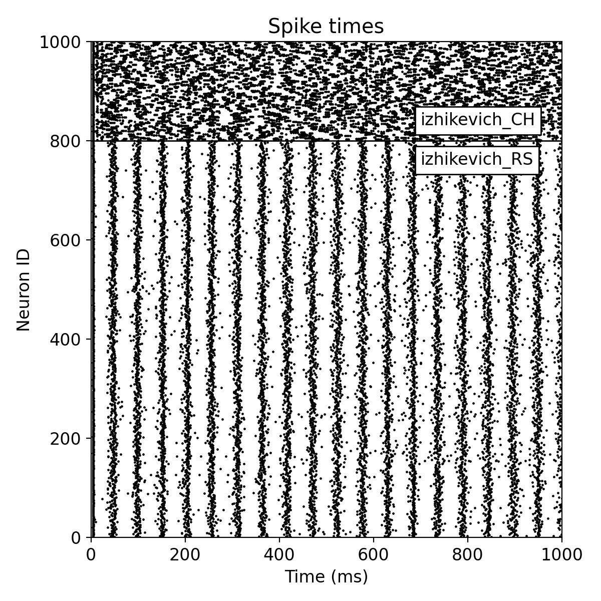
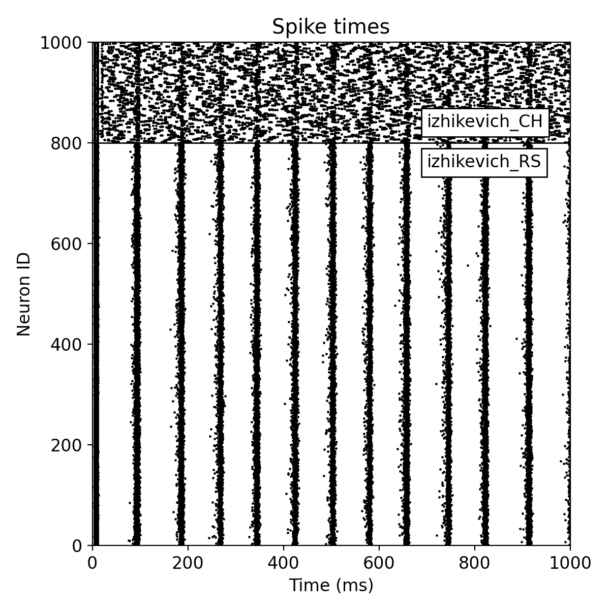
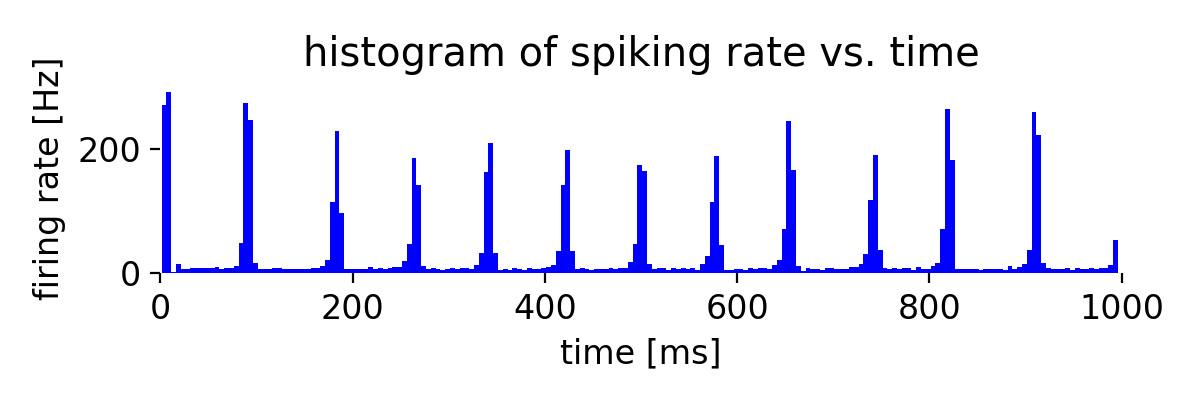
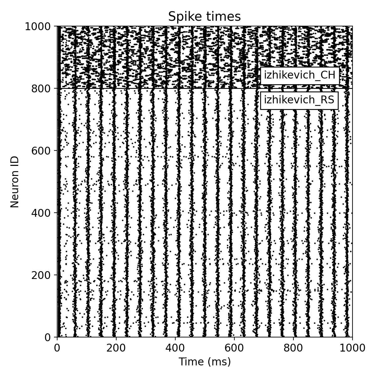
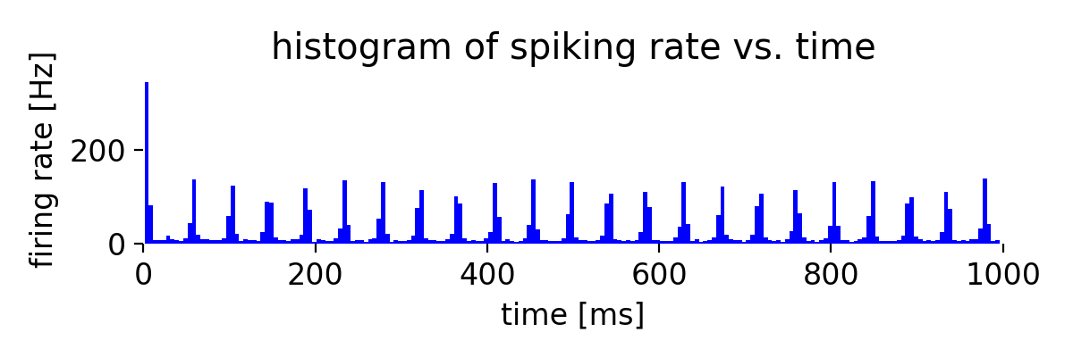
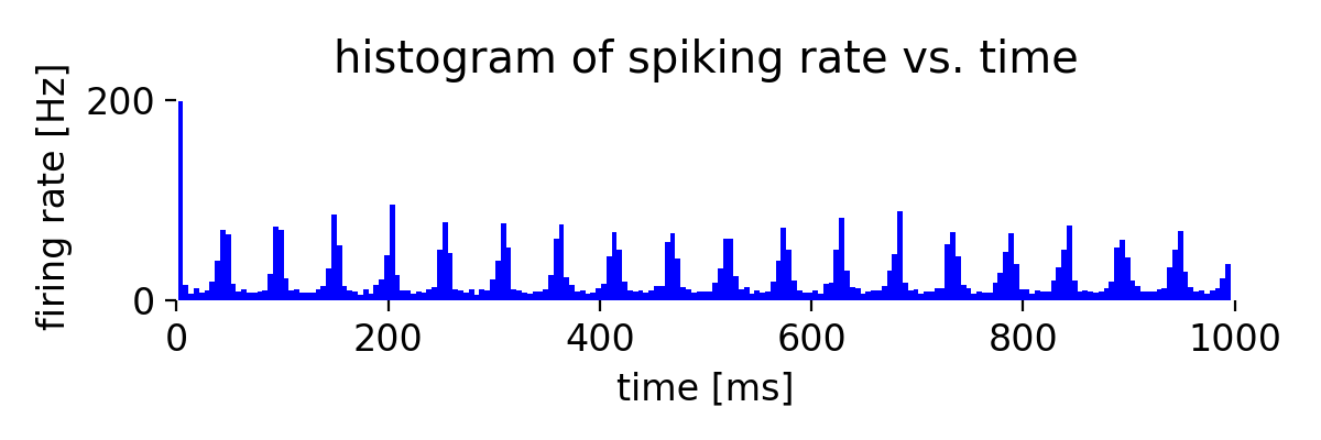Simulation results for two neuron populations of Izhikevich neurons of 800 regular spiking (RS) and 200 chattering (CH) neurons. The top panel shows the spike raster plot, and the bottom panel shows the histogram of the spiking rate vs. time.

The plot results show, how well the neurons in both populations synchronize their spiking activity. We also see the emerging oscillatory spiking behavior of the Izhikevich neurons. The regular spiking (RS) neurons show a more regular spiking pattern, while the spiking pattern of the chattering (CH) neurons is more irregular.

In the following, we briefly study the influence of various simulation parameters on the network dynamics.

Influence of the stimulation source

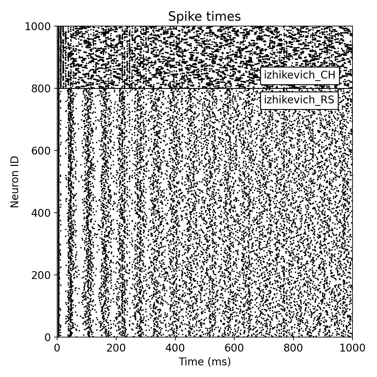
To assess the influence of the chosen stimulation source on the network dynamics, we run the simulation with a Poisson-noisy current input instead of the Gaussian-noisy current input:

# set up some Poisson-noisy current input:
noise = nest.Create("poisson_generator")
noise.rate = 5000.0 # [Hz]

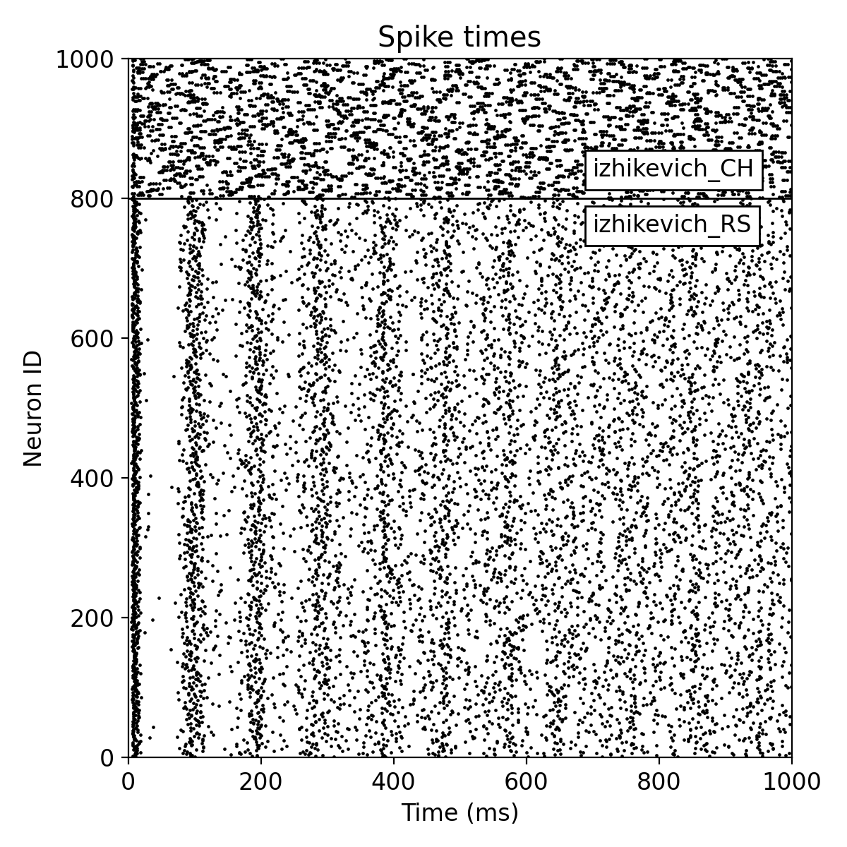
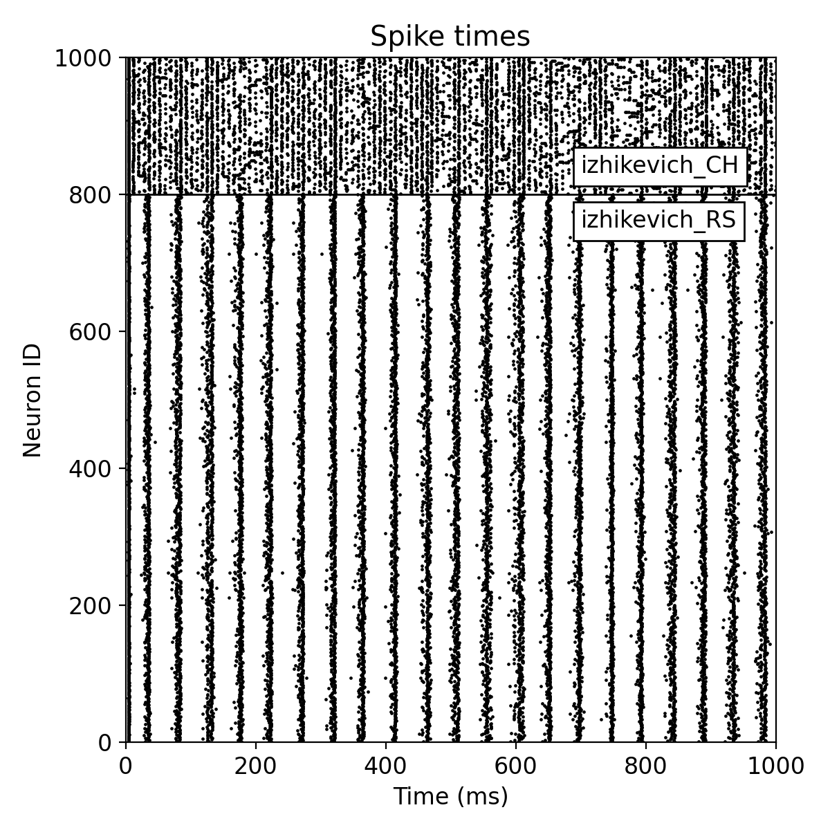
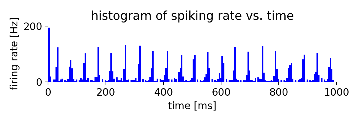
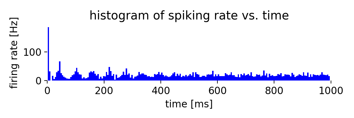
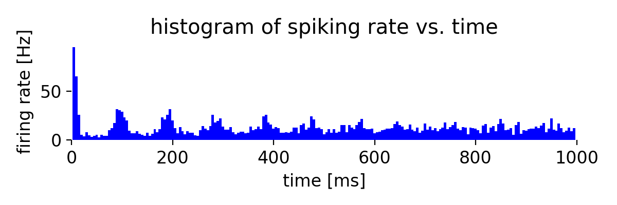Same simulation as before, but now with a Poisson noise generator as input source.

You can see, that the spiking activity of the neurons now contains more random spikes. However, the overall synchronization of the spiking activity is still maintained (for the regular spiking neurons).

Influence of the connection probability

A small change of the connection probability can have a significant impact on the network dynamics. For instance, changong the connection probability of the excitatory population to 20%,

conn_prob_ex = 0.20  # instead of 10%
conn_prob_in = 0.60

leads to a more synchronized spiking activity of the regular spiking neurons as well as the chattering neurons:

Same simulation as before, but now with a connection probability of 20% for the excitatory population.

Increasing the connection probability of the inhibitory population to 200%,

conn_prob_ex = 0.10
conn_prob_in = 2.0  # instead of 0.60

leads to a more synchronized spiking activity of the chattering neurons:

Same simulation as before, but now with a connection probability of 200% for the inhibitory population.

The type of connection rule itself can also have a significant impact on the network dynamics. For instance, changing the connection rule from a random fixed indegree to a random fixed outdegree connectivity,

conn_dict_ex_to_ex = {"rule": "fixed_outdegree", "outdegree": num_conn_ex_to_ex}
conn_dict_ex_to_in = {"rule": "fixed_outdegree", "outdegree": num_conn_ex_to_in}
conn_dict_in_to_ex = {"rule": "fixed_outdegree", "outdegree": num_conn_in_to_ex}
conn_dict_in_to_in = {"rule": "fixed_outdegree", "outdegree": num_conn_in_to_in}

will impact the synchronization of the spiking activity of the neurons:

Same simulation as before, but now with a random fixed outdegree connectivity.

Influence of the synaptic weights

The synaptic weights can also have a significant impact on the network dynamics. For instance, changing the synaptic weight of the inhibitory connections to -2.0,

# synaptic weights and delays:
d = 1.0 # synaptic delay [ms]
syn_dict_ex = {"delay": d, "weight": 0.5}
syn_dict_in = {"delay": d, "weight": -2.0}  # instead of -1.0

will alter the synchronization of the spiking activity of the neurons and increase the synchronization of the chattering neurons:

Same simulation as before, but now with a synaptic weight of -2.0 for the inhibitory connections.

Conclusion

NEST is a powerful and flexible simulator that allows for the simulation of large-scale, multi-population spiking neural networks with ease. In this post, we have explored how to set up a simple SNN simulation consisting two distinct populations of Izhikevich neurons. We have shown how to create parameterized populations of neurons, randomize the parameters of the neurons, and connect the populations of neurons. We have also discussed the influence of various simulation parameters such as the stimulation source, connection probability, connection rule, and synaptic weights on the network dynamics. The results of the simulations show how well the neurons on both populations synchronize their spiking activity and how the different neuron types exhibit distinct spiking patterns.

The complete code used in this blog post is available in this Github repositoryꜛ. Feel free to modify and expand upon it, and share your insights.