Izhikevich model

Computational neuroscience utilizes mathematical models to understand the complex dynamics of neuronal activity. Among various neuron models, the Izhikevich model stands out for its ability to combine biological fidelity with computational efficiency. Developed by Eugene Izhikevich in 2003ꜛ, this model simulates the spiking and bursting behavior of neurons with a remarkable balance between simplicity and biological relevance. In this post, we explore the properties of the Izhikevich model, examining its application and adaptability in simulating single neuron behaviors.

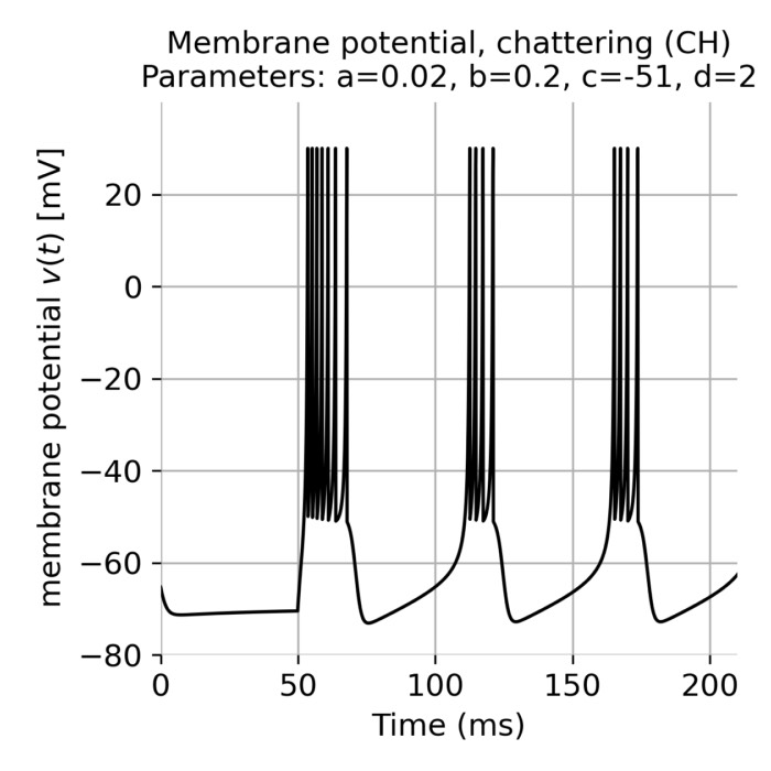Izhikevich Neuron Model: Example of chattering neuron.

Mathematical foundation

The Izhikevich model bridges the gap between detailed biophysical models like the Hodgkin-Huxley model and more abstract models like the Integrate-and-Fire model. While the former is biologically realistic but computationally expensive, the latter is computationally efficient but biologically unrealistic and lacks the ability to reproduce the rich dynamics of real neurons. In contrast, the Izhikevich model offers a compromise by capturing essential neuronal dynamics with a reduced set of equations. This reduction, based on bifurcation methodologies, allows for faster simulations while retaining essential features of neuronal dynamics.

The model is defined by a two-dimensional system of ordinary differential equations (ODE),

\[\begin{align} \frac{dv}{dt} &= 0.04v^2 + 5v + 140 - u + I \label{eq:model1} \\ \frac{du}{dt} &= a(bv - u) \label{eq:model2} \end{align}\]

along with an after-spike reset condition:

\[\begin{align} \text{if } v \geq 30 \text{ mV, then } & \begin{cases} v \leftarrow c \\ u \leftarrow u + d \end{cases} \label{eq:reset} \end{align}\]

The variable $v$ represents the membrane potential, and $u$ is a recovery variable that provides negative feedback to $v$. Both variables are dimensionless. $I$ is the synaptic or injected current. $a$, $b$, $c$, and $d$ are dimensionless parameters that define neuron dynamics, and they can be tuned to replicate various types of neuronal behaviors. In particular,

• $a$ controls the time scale of the recovery variable $u$, with smaller values leading to slower recovery.
• $b$ determines the sensitivity of the recovery variable $u$ to the subthreshold fluctuations of membrane potential $v$. Larger values result in a stronger coupling between $v$ and $u$, which possibly leads to subthreshold oscillations and low-threshold spiking behavior.
• $c$ is the after-spike reset value of the membrane potential $v$.
• $d$ is the increment of the recovery variable $u$ after a spike. It mimics the slow recovery of the membrane potential after an action potential.

The following plot visualizes the effect of the four parameters on the dynamics of the Izhikevich model:

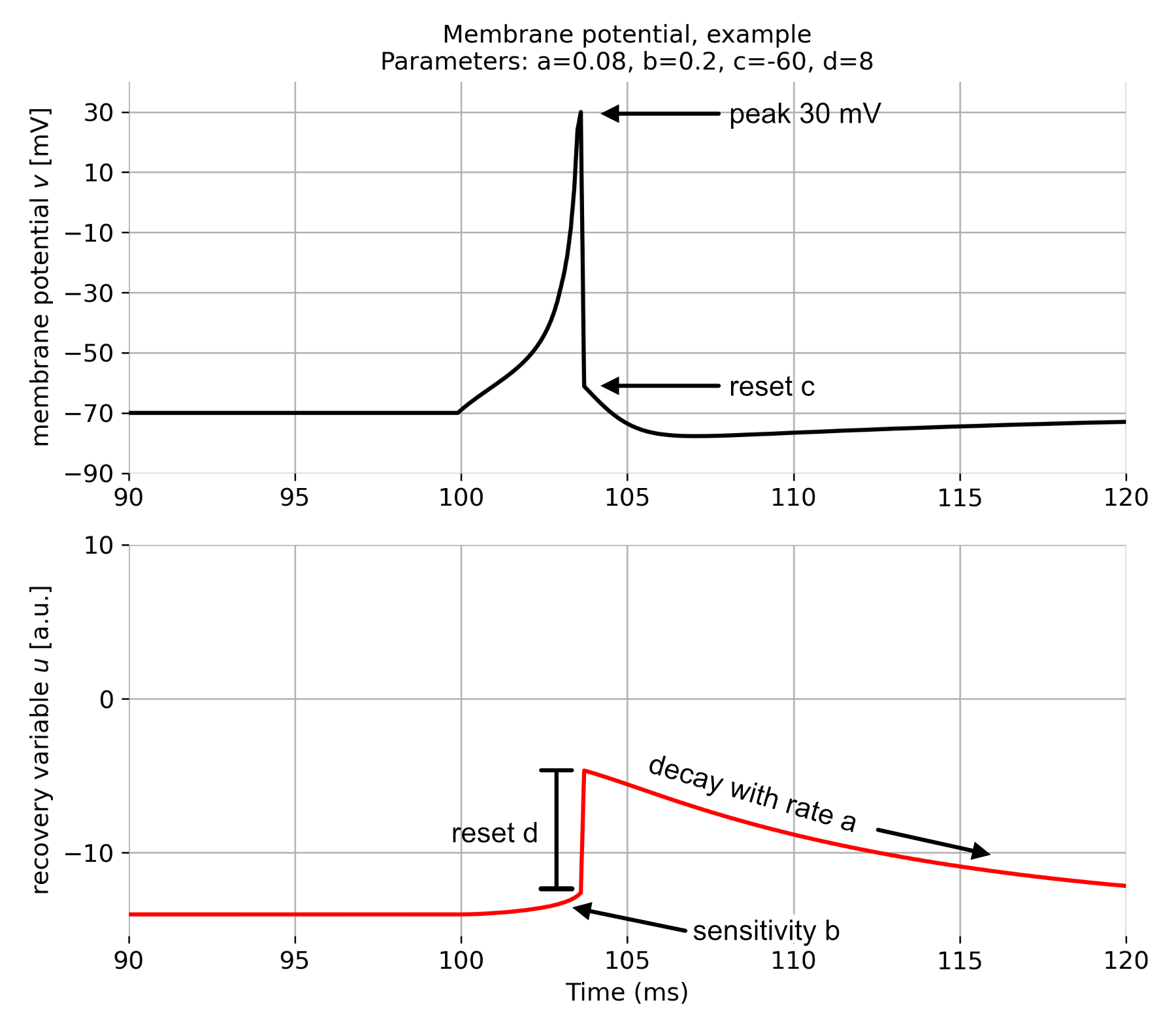
Membrane potential $v$ (top) and recovery variable $u$ (bottom) of a regular spiking neuron simulated using the Izhikevich model. Indicated are the parameters $a$, $b$, $c$, and $d$. To simulate the action potential, we set $a=0.08$, $b=0.2$, $c=-60$, and $d=8$. A current of $I=10$ was applied for 3 ms from 100 to 103 ms. Own illustration based on Fig. 2. from Izhikevich (2003)ꜛ.

The specific numbers in Eq. ($\ref{eq:model1}$), $0.04v^2 + 5v + 140$, result from fitting the spike generation dynamics to experimental data of cortical neurons so that the membrane potential $v$ has the scale of mV and the time $t$ has the scale of ms. Other choices of the parameters in Eq. ($\ref{eq:model1}$) are also possible to model different types of neurons.

Eq. ($\ref{eq:model1}$) and ($\ref{eq:model2}$) describe the evolution of the membrane potential and recovery variable over time. The reset condition Eq. ($\ref{eq:reset}$) ensures the model generates realistic action potentials by resetting the membrane potential and adjusting the recovery variable whenever the potential reaches a peak of 30 mV. The Izhikevich model is particularly well-suited for exploring the diverse behaviors of different types of neurons, including regular spiking, fast spiking, and bursting neurons as we will explore in the following sections.

Python code

To simulate the model, we choose the Euler method for numerical integration similar to Izhikevich’s original paper. However, we modify the code in such a way that the integration is performed with an adjustable step size dt. Choosing a smaller step size $\lt$1 will increase the accuracy of the simulation but also increase the computational cost. A value of dt=0.1 is a good starting point for most simulations with a good balance between accuracy and computational efficiency.

In the code, different sets of parameters are pre-defined for various neuron types, that we will discuss in more detail in the next section. By changing the parameter set, you can simulate different types of neurons. The code also allows you to adjust the input current I_baseline over time as well as the start and end time of the input current.

For plotting the membrane potential $v$, we clip the values to a maximum of 30 mV to visualize realistic action potentials.

import numpy as np
import matplotlib.pyplot as plt

# set simulation time and time step size:
T       = 400  # total simulation time in ms
dt      = 0.1  # time step size in ms
steps   = int(T / dt)  # number of simulation steps
t_start = 50  # start time for the input current
t_end   = T  # end time for the input current

# initialize parameters for one excitatory neuron:
p_RS  = [0.02, 0.2, -65, 8, "regular spiking (RS)"] # regular spiking settings for excitatory neurons (RS)
p_IB  = [0.02, 0.2, -55, 4, "intrinsically bursting (IB)"] # intrinsically bursting (IB)
p_CH  = [0.02, 0.2, -51, 2, "chattering (CH)"] # chattering (CH)
p_FS  = [0.1, 0.2, -65, 2, "fast spiking (FS)"] # fast spiking (FS)
p_TC  = [0.02, 0.25, -65, 0.05, "thalamic-cortical (TC)"] # thalamic-cortical (TC) (doesn't work well)
p_LTS = [0.02, 0.25, -65, 2, "low-threshold spiking (LTS)"] # low-threshold spiking (LTS)
p_RZ  = [0.1, 0.26, -65, 2, "resonator (RZ)"] # resonator (RZ)
a, b, c, d, type = p_RS # just change the parameter set here to simulate different neuron types

# initial values of v and u:
v = -65 # mV
u = b * v

# initialize array to store the u, v, I and t values over time:
u_values = np.zeros(steps)
v_values = np.zeros(steps)
I_values = np.zeros(steps)
t_values = np.zeros(steps)

# set the baseline current:
I_baseline = 10 # nA

# simulation:
for t in range(steps):
    t_ms = t * dt  # current time in ms

    if t_ms >= t_start and t_ms <= t_end:
        I = I_baseline 
    else:
        I = 0

    # check for spike and reset if v >= 30 mV (reset-condition):
    if v >= 30:
        v = c  # reset membrane potential v to c
        u += d # increase recovery variable u by d

    # Euler's method for numerical integration:
    v += dt * 0.5 * (0.04 * v**2 + 5 * v + 140 - u + I)
    v += dt * 0.5 * (0.04 * v**2 + 5 * v + 140 - u + I)
    u += dt * a * (b * v - u)

    # store values for plotting:
    u_values[t] = u
    v_values[t] = v
    I_values[t] = I
    t_values[t] = t_ms

# ensure v_values do not exceed 30 mV in the plot:
v_values = np.clip(v_values, None, 30)

# plotting:
fig, ax1 = plt.subplots(figsize=(8,3.85))

# plot v_values on the left y-axis:
ax1.plot(t_values, v_values, label='Membrane potential v(t)', color='k', lw=1.3)
ax1.set_xlabel('Time (ms)')
ax1.set_ylabel('membrane potential $v$ [mV]', color='k')
ax1.tick_params(axis='y', colors='k')

# create a second y-axis for u_values:
ax2 = ax1.twinx()
ax2.plot(t_values, u_values, label='Recovery variable u(t)', color='r', lw=2, alpha=1.0)
ax2.set_ylabel('recovery variable $u$ [a.u.]', color='r')
ax2.tick_params(axis='y', colors='r')
ax2.set_ylim(-20, 10)

# create a third y-axis for I_values:
ax3 = ax1.twinx()
ax3.spines['right'].set_position(('outward', 60))  
ax3.plot(t_values, I_values, label='Input Current I(t)', color='b', lw=2, alpha=0.75)
ax3.set_ylabel('input current $I$ [nA]', color='b')
ax3.tick_params(axis='y', colors='b')
ax3.set_ylim(-1,60)
ax3.set_frame_on(True)
ax3.patch.set_visible(False)

plt.title(f'Membrane potential, recovery variable, and input current, {type}\n'
            f"Parameters: a={a}, b={b}, c={c}, d={d}", fontsize=12)
plt.tight_layout()
plt.show()

The code above shows the core concept of the Izhikevich model simulation. The entire code can be found in this Github repositoryꜛ.

Simulating different neuron types

The Izhikevich model can simulate various types of neurons by adjusting the parameters $a$, $b$, $c$, and $d$. Here are some examples of different neuron types and their corresponding parameter sets that can be found in the mammalian neocortex:

Regular spiking neurons

The most common type of excitatory neuron in the neocortex are regular spiking (RS) neurons. They are characterized by a regular firing pattern when exposed to a constant input current, showing a short inter-spike interval at the beginning which increases over time. This behavior is also called spike frequency adaptation. An increase in the input current will increase the the inter-spike frequency. However, RS neurons will never fire at high frequencies due to the the large spike-afterhyperpolarization. The parameters for RS neurons are $a=0.02$, $b=0.2$, $c=-65$, and $d=8$. $c=-65$ corresponds to a large voltage reset after a spike, and $d=8$ corresponds to a large after-spike increase of the recovery variable $u$.

Membrane potential $v$ (black line), recovery variable $u$ (red) and applied input current $I$ (bl) of a regular spiking (RS) neuron simulated using the Izhikevich model. The parameters $a=0.02$, $b=0.2$, $c=-65$, and $d=8$ were used.

Same simulation as before, but using a higher input current of $I=20$ nA. The neuron fires at a higher frequency due to the increased input current, but still shows spike frequency adaptation and, thus, will not reach high firing frequencies compared to, e.g, fast spiking neurons (see below).

Intrinsically bursting neurons

Intrinsically bursting (IB) neurons are characterized by a burst of action potentials followed by repetitive single spikes. The parameters for IB neurons are $a=0.02$, $b=0.2$, $c=-55$, and $d=4$. During the initial burst, the recovery variable $u$ increases rapidly and then switches to (regular) spiking dynamics.

Membrane potential $v$ (black line), recovery variable $u$ (red) and applied input current $I$ (bl) of an intrinsically bursting (IB) neuron simulated using the Izhikevich model. The parameters $a=0.02$, $b=0.2$, $c=-55$, and $d=4$ were used. A pronounced burst of action potentials after the onset of the constant input current is followed by a series of single spikes.

Chattering neurons

Chattering (CH) neurons are characterized by bursts of closely spaced action potentials followed by a hyperpolarization. The inter-burst frequency can reach high values up to 40 Hz. The parameters for CH neurons are $a=0.02$, $b=0.2$, $c=-51$ tp $-50$, and $d=2$. The lower value of $d$ compared to IB and RS neurons results in a slower recovery of the membrane potential after a burst.

Membrane potential $v$ (black line), recovery variable $u$ (red) and applied input current $I$ (bl) of a chattering (CH) neuron simulated using the Izhikevich model. The parameters $a=0.02$, $b=0.2$, $c=-51$, and $d=2$ were used. The neuron shows a series of bursts of action potentials each directly followed by an extended hyperpolarization phase.

Fast spiking neurons

Fast spiking (FS) neurons are one of two types of inhibitory neurons in the cortex. They fire periodic trains of action potentials at high frequencies with almost no adaptation, i.e., no slowing down of the firing rate. The parameters for FS neurons are $a=0.1$, $b=0.2$, $c=-65$, and $d=2$. The higher value of $a$ compared to RS neurons results in a faster recovery of the membrane potential.

Membrane potential $v$ (black line), recovery variable $u$ (red) and applied input current $I$ (bl) of a fast spiking (FS) neuron simulated using the Izhikevich model. The parameters $a=0.1$, $b=0.2$, $c=-65$, and $d=2$ were used. The neuron exhibits tonic firing with, i.e., trains of action potentials at high frequencies with almost no adaptation.

Low-threshold spiking neurons

Low-threshold spiking (LTS) neurons are the second type of inhibitory neurons in the cortex. Similar to FS neurons, they fire periodic trains of action potentials at high frequencies. However, LTS neurons exhibit spike-frequency adaptation, leading to a decrease in the firing rate over time. These neurons also exhbit a low-threshold for spiking and can be simulated with the parameters $a=0.02$, $b=0.25$, $c=-65$, and $d=2$. $b=0.25$ accounts for the low-threshold spiking behavior.

Membrane potential $v$ (black line), recovery variable $u$ (red) and applied input current $I$ (bl) of a low-threshold spiking (LTS) neuron simulated using the Izhikevich model. The parameters $a=0.02$, $b=0.25$, $c=-65$, and $d=2$ were used. The neuron shows a series of action potentials at high frequencies with spike-frequency adaptation.

Thalamic-cortical neurons

The model is also able to simulate thalamic-cortical (TC) neurons, which are found in the thalamus and project to the cortex. TC neurons provide the major input to the cortex and are involved in the generation of sleep rhythms. They have two firing modes. First, when exposed to a constant positive input current, they exhibit a tonic firing pattern. Second, when exposed to a negative input current which abruptly switches to 0, the TC neurons fire a rebound of action potentials. The parameters for TC neurons are $a=0.02$, $b=0.25$, $c=-65$, and $d=0.05$.

Membrane potential $v$ (black line), recovery variable $u$ (red) and applied input current $I$ (bl) of a thalamic-cortical (TC) neuron simulated using the Izhikevich model. The parameters $a=0.02$, $b=0.25$, $c=-65$, and $d=0.05$ were used. The neuron shows a tonic firing pattern when exposed to a constant positive input current.

When exposed to a negative input current which abruptly switches to 0, the TC neuron fires a rebound of action potentials.

Resonator neurons

In his original paper, Izhikevich shows that the model is able to simulate another interesting type of neurons: Resonator (RZ) neurons. These neurons are able to resonate to rhythmic inputs that have an appropriate frequency. As far as I understand, the model mimics this behavior by exhibiting subthreshold oscillations in response to a constant input current. Furthermore, the neuron would switch to repetitive spiking when exposed to a short-term input current pulse. The corresponding parameters for RZ neurons are $a=0.1$, $b=0.26$, $c=-65$, and $d=2$. However, I was not able to reproduce the resonator behavior with these parameters. I tried different values and different input currents, without success. If you have any suggestions on how to simulate the resonator behavior, please let me in the comments below.

Summary of parameters for different neuron types

The following plot summarizes the different parameter sets for the various neuron types described above:

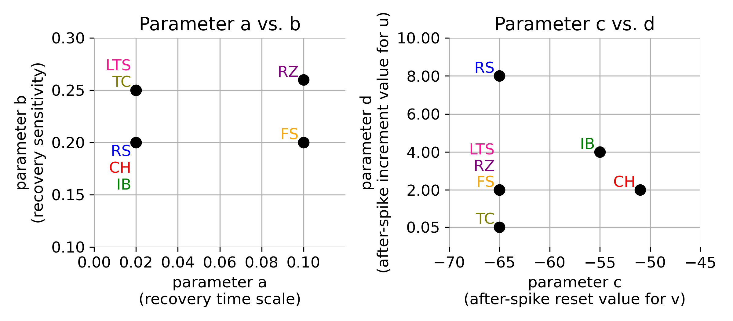
Parameter space of $a$, $b$, $c$ and $d$ for different neuron types. The parameter sets for regular spiking (RS), intrinsically bursting (IB), chattering (CH), fast spiking (FS), low-threshold spiking (LTS), thalamic-cortical (TC), and resonator (RZ) neurons are indicated. Own illustration based on Fig. 2. from Izhikevich (2003)ꜛ.

Conclusion

The Izhikevich model is a powerful tool for simulating the spiking and bursting behavior of neurons with a remarkable balance between simplicity and biological relevance. By adjusting the parameters $a$, $b$, $c$, and $d$, the model can simulate various types of neurons found in the mammalian neocortex, including regular spiking, fast spiking, and bursting neurons, while being computationally efficient.

Despite its advantages, the Izhikevich model is not without limitations. The model can oversimplify certain neuronal behaviors, particularly those involving complex ion channel dynamics and second messenger systems. Furthermore, the model’s reliance on parameter tuning for different neuron types can make it less predictive compared to more detailed models.

Nevertheless, the Izhikevich model serves as a bridge between biologically detailed, computationally demanding models and more abstract, simplified neuronal models. It provides a versatile platform for exploring neuronal behavior and network dynamics with considerable ease and efficiency. In the next post we will discover, how the Izhikevich model can be used to efficiently simulate networks of spiking neurons.

The complete code used in this blog post is available in this Github repositoryꜛ. Feel free to experiment with it, modify the parameters, and explore the dynamics of the Izhikevich model further. And for any ideas regarding the not yet solved resonator behavior, please leave a comment below.

References and further reading

• Izhikevich, Simple model of spiking neurons, 2003, IEEE Transactions on Neural Networks, Vol. 14, Issue 6, pages 1569-1572, doi: 10.1109/TNN.2003.820440ꜛ, PDFꜛ
• Izhikevich, Eugene M., (2010), Dynamical systems in neuroscience: The geometry of excitability and bursting (First MIT Press paperback edition), The MIT Press, ISBN: 978-0-262-51420-0, PDFꜛ