t-SNE and PCA: Two powerful tools for data exploration

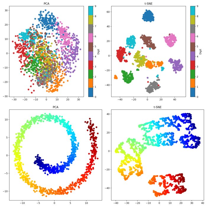
Dimensionality reduction techniques play a vital role in both data exploration and visualization. Among these techniques, t-Distributed Stochastic Neighbor Embedding (t-SNE) and Principal Component Analysis (PCA) are widely used and offer valuable insights into complex datasets. In this blog post, we explore te mathematical background of both methods, compare their methodologies, and discuss the advantages and disadvantages of each. Additionally, we take a look at their practical implementation in Python and compare the results on different sample datasets.

Mathematical Background

t-SNE and PCA both leverage mathematical principles to reduce the dimensionality of data. Let’s briefly outline the key mathematical components of each technique.

t-SNE

t-SNE is based on the concept of probability distributions and similarity between data points. Given a high-dimensional dataset with N points, t-SNE constructs probability distributions P and Q over pairs of points in the original space and the embedding space, respectively.

To measure similarity, t-SNE employs the Gaussian kernel:

\[p_{j|i} = \frac{\exp(-\lVert x_i - x_j \rVert^2 / (2 \sigma_i^2))}{\sum_{k \neq i} \exp(-\lVert x_i - x_k \rVert^2 / (2 \sigma_i^2))}\]

Here, \(x_i\) and \(x_j\) represent data points in the original space, \(\sigma_i\) is the variance of the Gaussian distribution centered at \(x_i\), and \(p_{j\vert i}\) denotes the conditional probability of \(x_j\) given \(x_i\).

The objective of t-SNE is to minimize the Kullback-Leibler ($KL$) divergence between the distributions $P$ and $Q$:

\[KL(P || Q) = \sum_{i,j} p_{ij} \log \frac{p_{ij} }{q_{ij} }\]

Here, $p_{ij}$ and $q_{ij}$ represent the joint probabilities of pairs of points in the original and embedding space, respectively.

PCA

PCA, on the other hand, is a statistical technique that aims to capture the directions of maximum variance in the data. It accomplishes this by performing an eigendecomposition of the covariance matrix of the data.

Given a dataset of $N$ data points, each consisting of $d$-dimensional feature vectors, PCA seeks to find a set of orthogonal axes, known as principal components, that represent the directions of maximum variance in the data.

The steps involved in PCA are as follows:

1. Mean Centering

PCA begins by subtracting the mean of each feature from the corresponding data points. This step ensures that the data is centered around the origin, eliminating any bias due to differing means across features.

2. Covariance Matrix

Next, PCA computes the covariance matrix of the mean-centered data. The covariance matrix is a $d \times d$ symmetric matrix that quantifies the relationships and variances between pairs of features.

The covariance matrix is defined as:

\[C = \frac{1}{N-1}(X - \mu)^T(X - \mu)\]

Here, $C$ represents the covariance matrix, $X$ is the mean-centered data matrix, $\mu$ is the mean vector, and $N$ is the number of data points.

Eigendecomposition

PCA performs an eigendecomposition of the covariance matrix. The eigendecomposition expresses the covariance matrix as a product of eigenvectors and eigenvalues.

The eigendecomposition is given by:

\[C = V \Lambda V^T\]

Here, $V$ represents the matrix of eigenvectors, and $\Lambda$ is a diagonal matrix containing the eigenvalues.

Dimensionality Reduction

Finally, PCA selects a subset of the principal components based on the desired number of dimensions or the desired amount of variance to be retained. The data can be projected onto these selected principal components, effectively reducing its dimensionality.

The transformed data obtained after projecting onto the principal components retains the most important information in terms of variance, allowing for effective visualization and analysis.

A practical demonstration of PCA can be found in this blog post.

Comparison and Advantages/Disadvantages

t-SNE and PCA differ significantly in their underlying methodologies and strengths. Let’s discuss their comparative advantages and disadvantages.

Advantages of t-SNE

1. Non-linear embedding: t-SNE excels at capturing non-linear relationships between data points, making it effective for visualizing complex structures and clusters that PCA might fail to capture.
2. Preservation of local structures: t-SNE emphasizes the preservation of local distances between neighboring points, revealing fine-grained details within clusters that might be lost in PCA’s global perspective.
3. Robustness to outliers: t-SNE is less sensitive to outliers compared to PCA since it focuses on local relationships rather than global variance.

Advantages of PCA

1. Computationally efficient: PCA is computationally less demanding compared to t-SNE, particularly for large datasets. It scales efficiently with the number of features.
2. Interpretable bomponents: PCA provides a direct mapping to the principal components, allowing for interpretation in terms of the original features or dimensions.
3. Effective for global structure: PCA is better suited for capturing the global structure of the data, especially when the primary goal is to capture the directions of maximum variance.

Python example 1

Below is a Python code snippet demonstrating the implementation of t-SNE and PCA, along with visualizations using a sample dataset. We utilized the Iris dataset for simplicity and the resulting plots showcase the transformed data points in the 2D space, with each point colored according to its class label.

import numpy as np
import matplotlib.pyplot as plt
from sklearn.datasets import load_iris, load_digits
from sklearn.datasets import make_swiss_roll
from sklearn.decomposition import PCA
from sklearn.manifold import TSNE

# Load the Iris dataset
iris = load_iris()
X, y = iris.data, iris.target

# Perform PCA
pca = PCA(n_components=2)
X_pca = pca.fit_transform(X)

# Perform t-SNE
tsne = TSNE(n_components=2)
X_tsne = tsne.fit_transform(X)

# Plot the results
plt.figure(figsize=(12, 6))
plt.subplot(121)
plt.scatter(X_pca[:, 0], X_pca[:, 1], c=y)
plt.title("PCA")
plt.subplot(122)
plt.scatter(X_tsne[:, 0], X_tsne[:, 1], c=y)
plt.title("t-SNE")
plt.show()

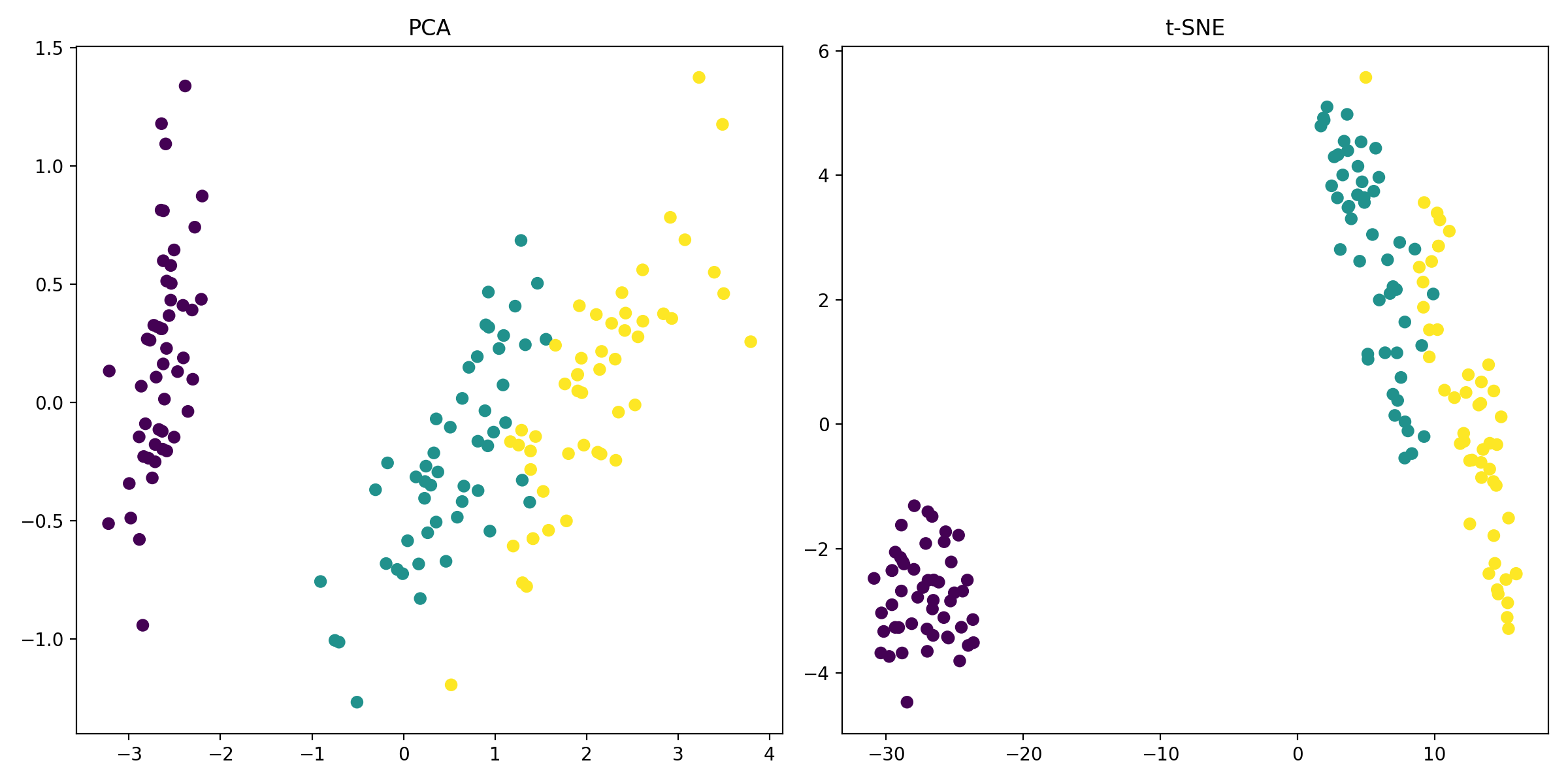PCA (left) and t-SNE (right) applied to the Iris dataset. The transformed data points are plotted in the 2D space, with each point colored according to its class label.

Python example 2

The next example is a bit complex, using the handwritten digits dataset:

# Load the handwritten digits dataset
digits = load_digits()
X, y = digits.data, digits.target

# Perform PCA
pca = PCA(n_components=2)
X_pca = pca.fit_transform(X)

# Perform t-SNE
tsne = TSNE(n_components=2)
X_tsne = tsne.fit_transform(X)

# Plot the results
plt.figure(figsize=(12, 6))
plt.subplot(121)
plt.scatter(X_pca[:, 0], X_pca[:, 1], c=y, cmap='tab10')
plt.colorbar(label='Digit')
plt.title("PCA")

plt.subplot(122)
plt.scatter(X_tsne[:, 0], X_tsne[:, 1], c=y, cmap='tab10')
plt.colorbar(label='Digit')
plt.title("t-SNE")

plt.tight_layout()
plt.savefig('pca_vs_tsne_2.png', dpi=200)
plt.show()

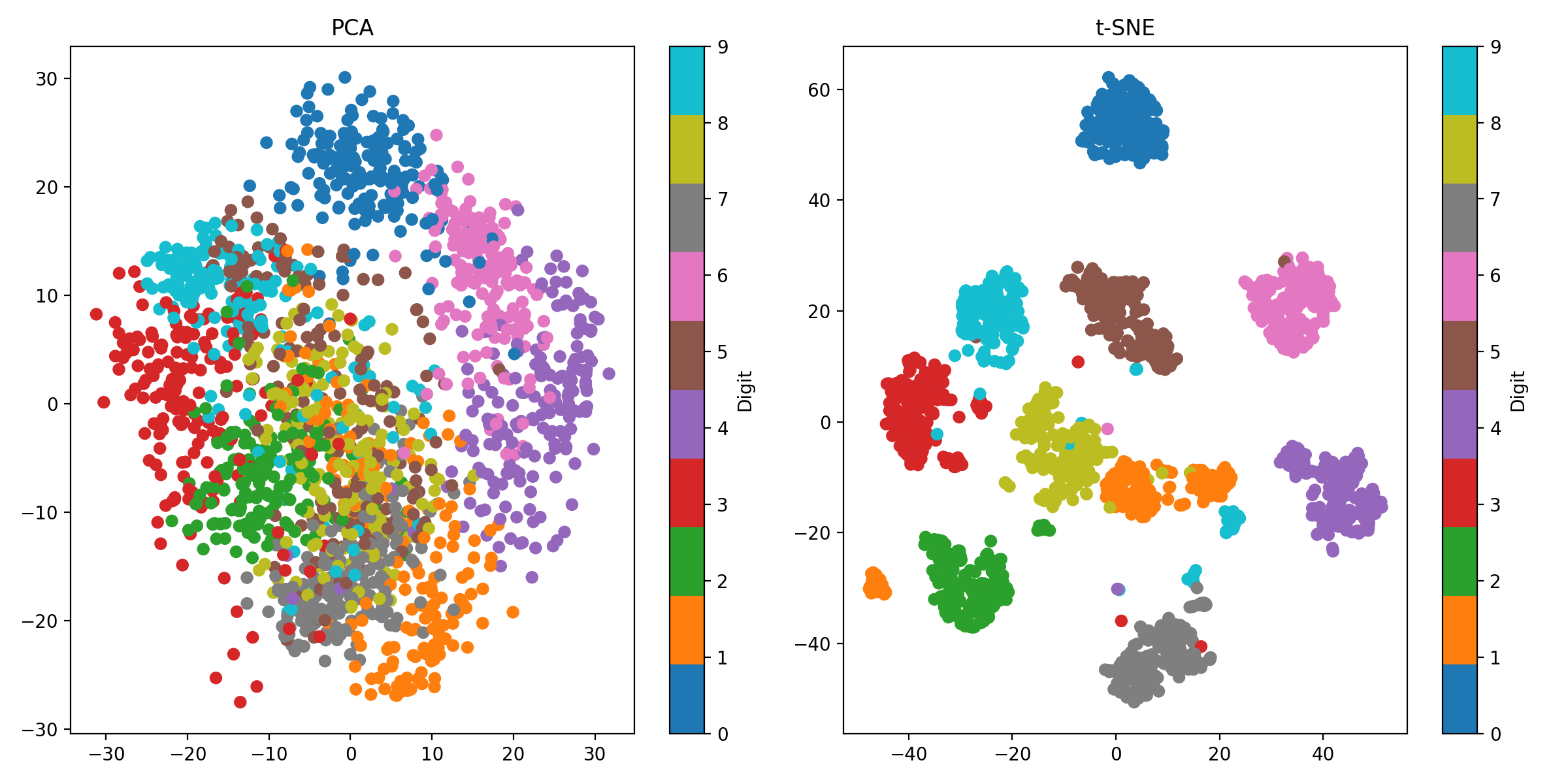PCA (left) and t-SNE (right) applied to the handwritten digits dataset. For this dataset, t-SNE is more effective at capturing the complex structures and clusters in the data.

Python example 3

Finally, we use the Swiss roll dataset to demonstrate the effectiveness of PCA in capturing the global structure of the data:

# Generate the Swiss Roll dataset
X, color = make_swiss_roll(n_samples=1500, noise=0.5, random_state=42)

# Perform PCA
pca = PCA(n_components=2)
X_pca = pca.fit_transform(X)

# Perform t-SNE
tsne = TSNE(n_components=2)
X_tsne = tsne.fit_transform(X)

# Plot the results
fig = plt.figure(figsize=(12, 6))

# Plot PCA results
ax1 = fig.add_subplot(121)
ax1.scatter(X_pca[:, 0], X_pca[:, 1], c=color, cmap='jet')
ax1.set_title("PCA")

# Plot t-SNE results
ax2 = fig.add_subplot(122)
ax2.scatter(X_tsne[:, 0], X_tsne[:, 1], c=color, cmap='jet')
ax2.set_title("t-SNE")

plt.tight_layout()
plt.savefig('pca_vs_tsne_3.png', dpi=200)
plt.show()

# plot the swiss roll:
fig = plt.figure(figsize=(6, 6))
ax = fig.add_subplot(111, projection='3d')
ax.scatter(X[:, 0], X[:, 1], X[:, 2], c=color, cmap='jet')
ax.view_init(8, -75)
plt.tight_layout()
plt.savefig('pca_vs_tsne_3_swissroll.png', dpi=200)
plt.show()

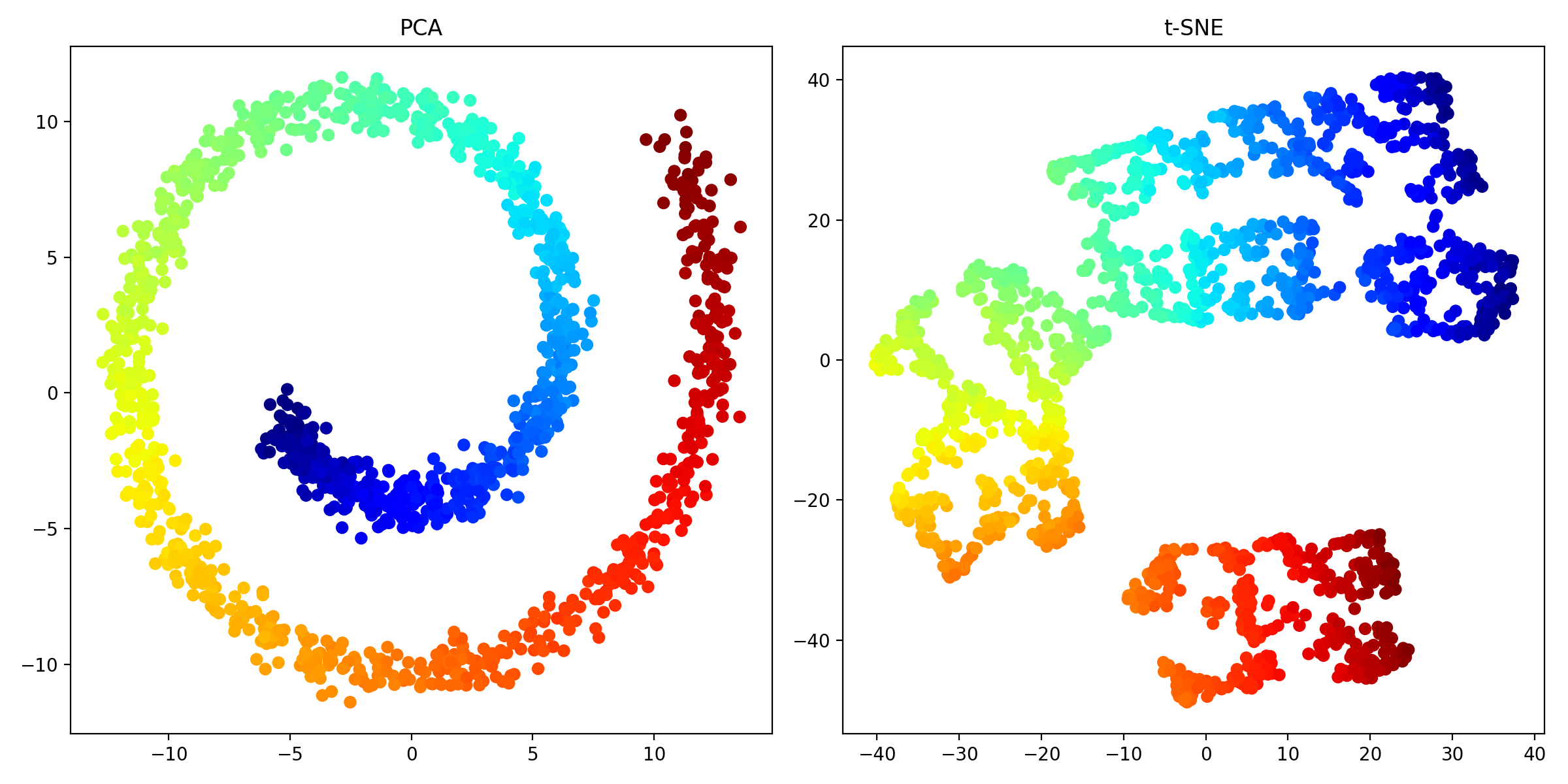PCA (left) and t-SNE (right) applied to the Swiss roll dataset. For this dataset, PCA is more effective at capturing the global structure of the data.

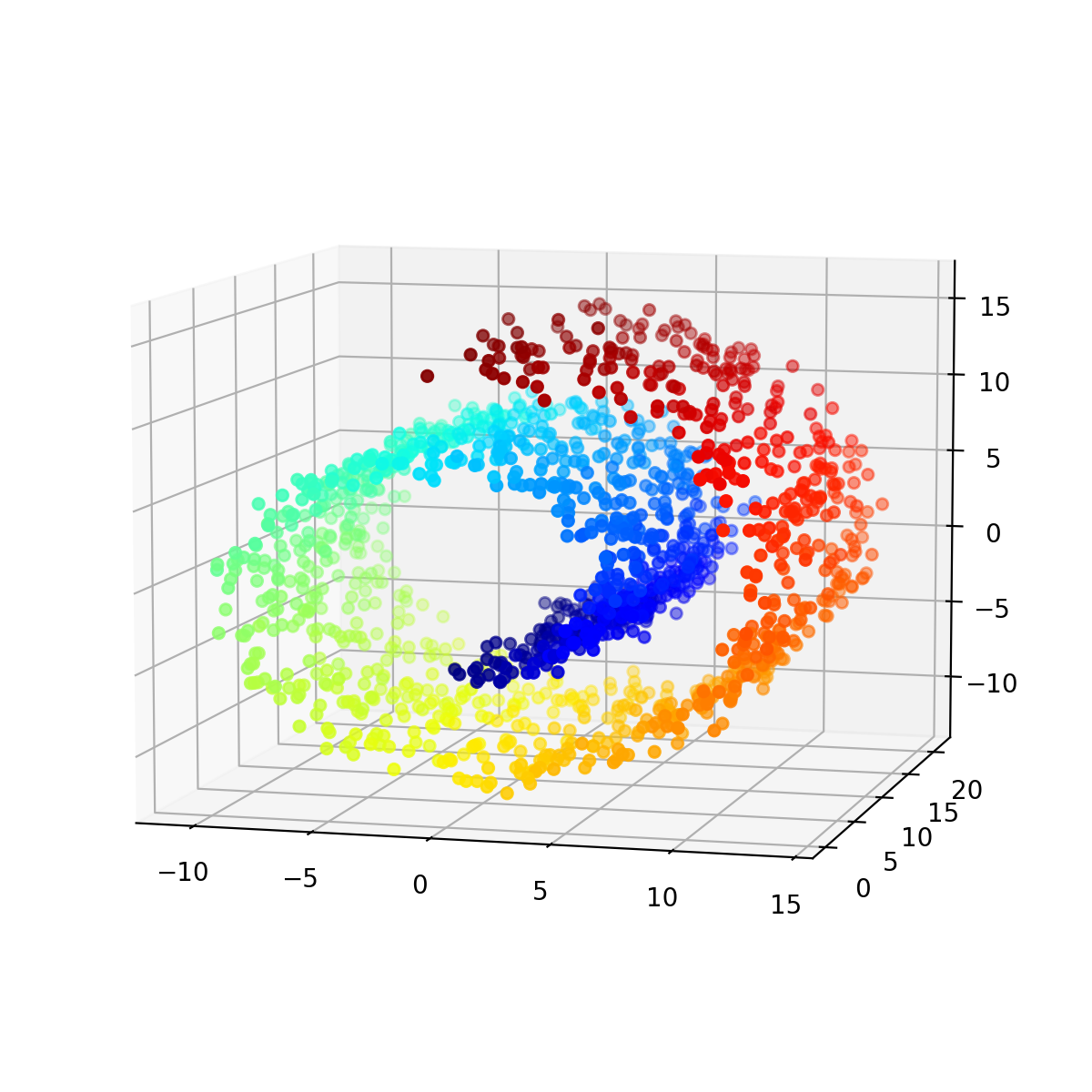
The Swiss roll dataset. The data points are colored according to their position along the roll.

Conclusion

t-SNE and PCA are powerful tools for data exploration and dimensionality reduction. While t-SNE excels at capturing complex, non-linear structures and preserving local relationships, PCA is more computationally efficient, provides interpretable components, and is effective for capturing global structures. By understanding the strengths and limitations of both techniques, you can employ them wisely to gain deeper insights into your datasets and facilitate data exploration in various domains.

The code used in this post is also available in this GitHub repositoryꜛ.

If you have any questions or suggestions, feel free to leave a comment below or reach out to me on Mastodonꜛ.