Understanding L1 and L2 regularization in machine learning

Regularization techniques play a vital role in preventing overfitting and enhancing the generalization capability of machine learning models. Among these techniques, L1 and L2 regularization are widely employed for their effectiveness in controlling model complexity. In this blog post, we explore the concepts of L1 and L2 regularization and provide a practical demonstration in Python.

Mathematical formulation

L1 regularization (Lasso)

L1 regularization, also known as Lasso regularization, adds a penalty term to the loss function of a model. It encourages the model to minimize the sum of absolute values of the coefficients (weights) in order to enforce sparsity. The L1 regularization term is represented as follows:

\[\text{L1 regularization term} = \lambda \sum_{j=1}^{p} |w_j|,\]

where $\lambda$ is the regularization parameter and $w_j$ represents the $j$-th coefficient.

L2 regularization (Ridge)

L2 regularization, also called Ridge regularization, adds a penalty term to the loss function that encourages the model to minimize the sum of squares of the coefficients. This regularization method constrains the coefficients to small values, thereby reducing the impact of individual features and preventing overfitting. The L2 regularization term can be expressed as:

\[\text{L2 regularization term} = \lambda \sum_{j=1}^{p} w_j^2.\]

Application to deep learning

Regularization acts on the weights of a model. In the context of deep learning, the weights of a neural network are the parameters that are learned during training. These parameters are adjusted by the network to minimize a loss function, which measures the discrepancy between the network’s predictions and the ground truth labels. The loss function is typically a function of the weights of the network, and regularization can be applied by adding a regularization term to the loss function \(\mathcal{L} = f(\mathbf{y}_\text{true}, \mathbf{y}_\text{pred})\), where \(\mathbf{y}_\text{true}\) represents the true labels of the training data and \(\mathbf{y}_\text{pred}\) represents the predicted labels produced by the neural network. The choice of the loss function depends on the specific task at hand, such as classification (e.g., cross-entropy loss) or regression (e.g., mean squared error). To incorporate regularization, we add the regularization term to the original loss function, which leads to the total loss function:

L1 regularization:

\[\mathcal{L}_\text{total} = \mathcal{L} + \lambda \sum_{i} |w_i|\]

L2 regularization:

\[\mathcal{L}_\text{total} = \mathcal{L} + \lambda \sum_{i} w_i^2\]

In both cases, the regularization term is added to the original loss function to create the total loss function, which the neural network aims to minimize during training. The regularization term acts as a penalty or constraint on the weights of the network, encouraging certain properties such as sparsity (in the case of L1) or smaller weights (in the case of L2).

Advantages and disadvantages

L1 regularization advantages

1. Feature selection: L1 regularization tends to yield sparse solutions, effectively performing feature selection by setting some coefficients to zero. This property is particularly valuable when dealing with high-dimensional datasets, as it helps identify the most important features.
2. Interpretable models: Due to the sparsity induced by L1 regularization, the resulting models are easier to interpret, as they focus on a subset of relevant features.

L1 regularization disadvantages

1. Non-differentiability: The L1 regularization term is non-differentiable at zero, which can make optimization more challenging compared to L2 regularization.
2. Unstable solutions: L1 regularization may produce unstable solutions when dealing with correlated features, as it tends to arbitrarily select one feature over another.

L2 regularization advantages

1. Stability: L2 regularization provides more stable solutions, especially in the presence of correlated features, as it shares the penalty among all coefficients rather than concentrating on a subset of features.
2. Computational efficiency: The L2 regularization term is differentiable, facilitating optimization algorithms to converge efficiently.

L2 regularization disadvantages

1. Lack of feature selection: Unlike L1 regularization, L2 regularization does not perform explicit feature selection, as it shrinks all coefficients towards zero rather than setting some to exactly zero.
2. Limited interpretability: The resulting models may involve all the available features, making them less interpretable compared to L1-regularized models.

Python code and plots

For our example, we will consider a deep learning network with multiple layers. Specifically, we will use a convolutional neural network (CNN) architecture. The CNN will consist of convolutional layers, followed by activation functions, pooling layers, and fully connected layers. We will apply L1 and L2 regularization separately to this network and compare their performance.

To evaluate the performance of L1 and L2 regularization in our deep learning network, we will train the network using a labeled dataset and monitor the loss curves of the training and validation datasets. The loss curve represents the decrease in the network’s loss (e.g., mean squared error) as training progresses.

For reproducibility:

conda create -n l1_l2_regularization python=3.9
conda activate l1_l2_regularization
conda install -y mamba
mamba install -y numpy matplotlib tensorflow

Here is the code:

import numpy as np
import matplotlib.pyplot as plt
import tensorflow as tf
from tensorflow.keras import datasets, layers, models

# Load the dataset
(train_images, train_labels), (test_images, test_labels) = datasets.cifar10.load_data()
train_images, test_images = train_images / 255.0, test_images / 255.0

# Define the CNN architecture
model = models.Sequential()
model.add(layers.Conv2D(32, (3, 3), activation='relu', input_shape=(32, 32, 3)))
model.add(layers.MaxPooling2D((2, 2)))
model.add(layers.Flatten())
model.add(layers.Dense(64, activation='relu'))
model.add(layers.Dense(10))

# Compile the model with L1 regularization
model_l1 = models.clone_model(model)
model_l1.set_weights(model.get_weights())
model_l1.add(layers.Dense(10, kernel_regularizer=tf.keras.regularizers.l1(0.01)))

# Compile the model with L2 regularization
model_l2 = models.clone_model(model)
model_l2.set_weights(model.get_weights())
model_l2.add(layers.Dense(10, kernel_regularizer=tf.keras.regularizers.l2(0.01)))

# Train the models
model.compile(optimizer='adam', loss=tf.keras.losses.SparseCategoricalCrossentropy(from_logits=True), metrics=['accuracy'])
model_l1.compile(optimizer='adam', loss=tf.keras.losses.SparseCategoricalCrossentropy(from_logits=True), metrics=['accuracy'])
model_l2.compile(optimizer='adam', loss=tf.keras.losses.SparseCategoricalCrossentropy(from_logits=True), metrics=['accuracy'])

history = model.fit(train_images, train_labels, epochs=10, validation_data=(test_images, test_labels))
history_l1 = model_l1.fit(train_images, train_labels, epochs=10, validation_data=(test_images, test_labels))
history_l2 = model_l2.fit(train_images, train_labels, epochs=10, validation_data=(test_images, test_labels))

# Plot the loss curves
plt.figure(figsize=(7, 6))
plt.plot(history.history['loss'], label='Training Loss (No Regularization)', 
         color='k', lw=2)
plt.plot(history.history['val_loss'], label='Validation Loss (No Regularization)', 
         color='k', ls='--', lw=2)
plt.xlabel('Epochs')
plt.ylabel('Loss')
plt.title('Comparison of Loss Curves (no regularization))')
plt.legend()
plt.xlim(-0.5, 9.5)
plt.ylim(0.7, 1.7)
plt.xticks(range(10))
plt.show()

plt.figure(figsize=(7, 6))
plt.plot(history_l1.history['loss'], label='Training Loss (L1 Regularization)', 
         color='#0072B2', lw=2)
plt.plot(history_l1.history['val_loss'], label='Validation Loss (L1 Regularization)', 
         color='#0072B2', ls='--', lw=2)
plt.xlabel('Epochs')
plt.ylabel('Loss')
plt.title('Comparison of Loss Curves (with L1 regularization)')
plt.legend()
plt.xlim(-0.5, 9.5)
plt.ylim(0.7, 1.7)
plt.xticks(range(10))
plt.show()

plt.figure(figsize=(7, 6))
plt.plot(history_l2.history['loss'], label='Training Loss (L2 Regularization)', 
         color='#E69F00', lw=2)
plt.plot(history_l2.history['val_loss'], label='Validation Loss (L2 Regularization)', 
         color='#E69F00', ls='--', lw=2)
plt.xlabel('Epochs')
plt.ylabel('Loss')
plt.title('Comparison of Loss Curves (with L2 regularization)')
plt.legend()
plt.xlim(-0.5, 9.5)
plt.ylim(0.7, 1.7)
plt.xticks(range(10))
plt.show()

Loss curves

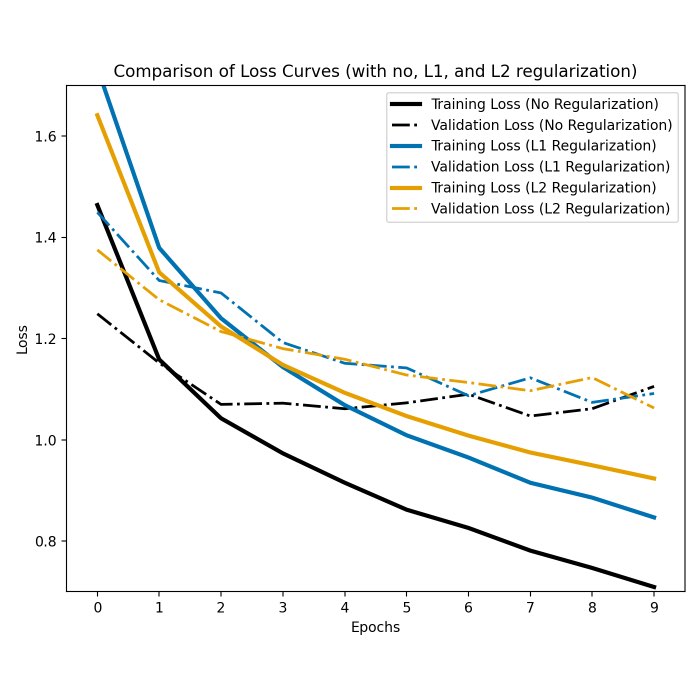
Without regularization, the model overfits the training data, as evidenced by the decreasing training loss and stagnating validation loss. This indicates that the model is unable to generalize to the validation data:

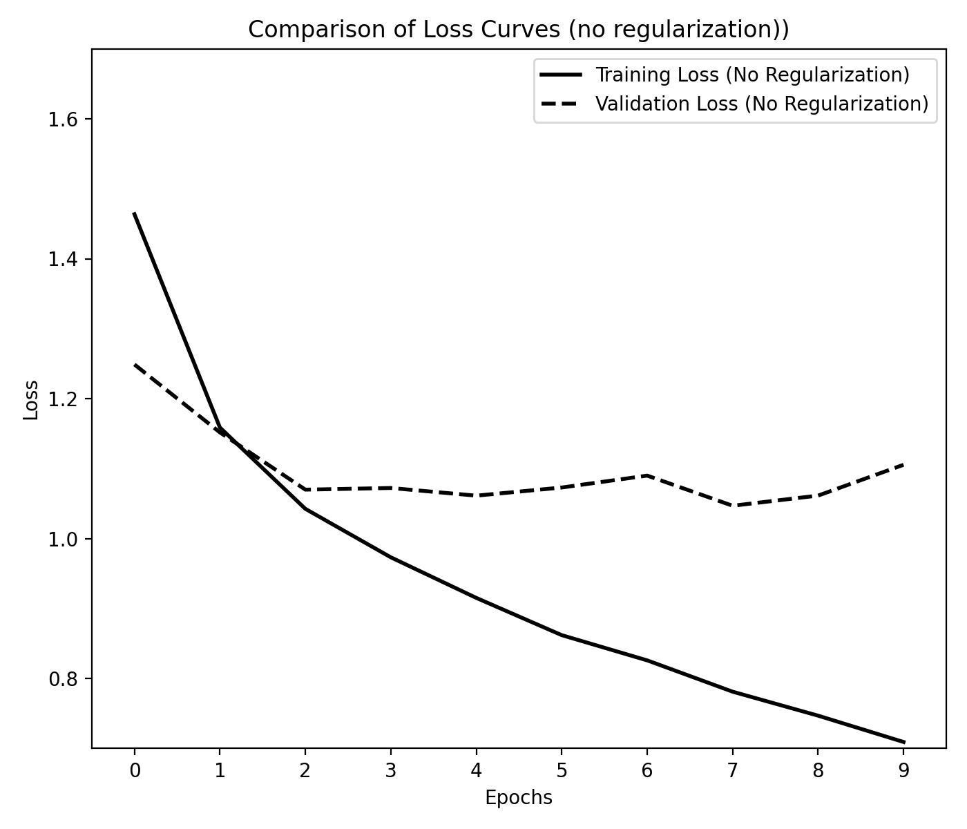Loss curves for the CNN without regularization. The training and validation losses are plotted as a function of the number of epochs. The model is trained for 10 epochs.

The L1 and L2 regularization terms are added to the loss function to penalize the weights of the network. This encourages the model to learn simpler representations and prevents overfitting. As a result, both the training loss and the validation loss decrease, indicating that the model is able to generalize to the validation data:

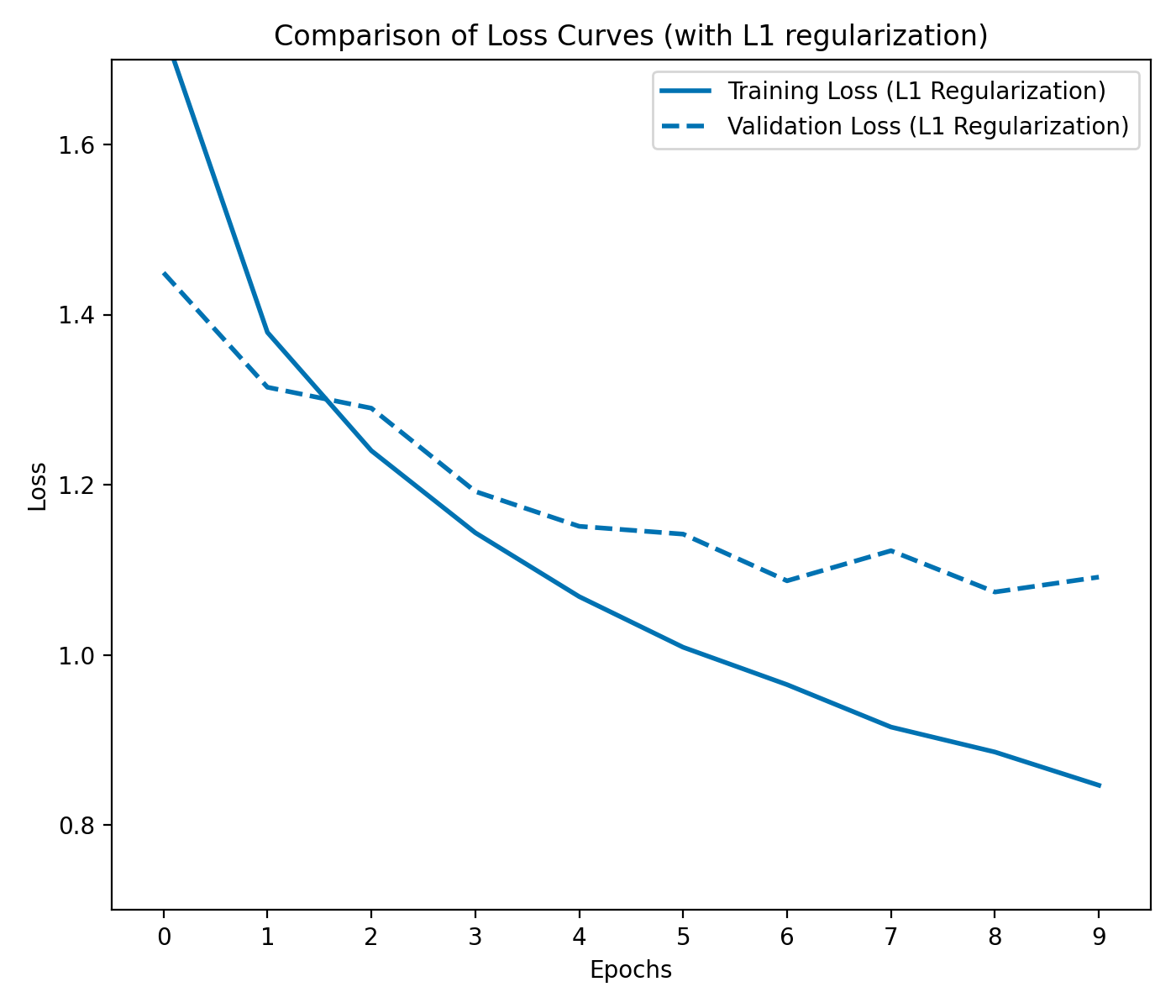Loss curves for the CNN with L1 regularization. Both, the training loss and validation loss decrease with each epoch, which is indicative of a model that is able to generalize to the validation data.

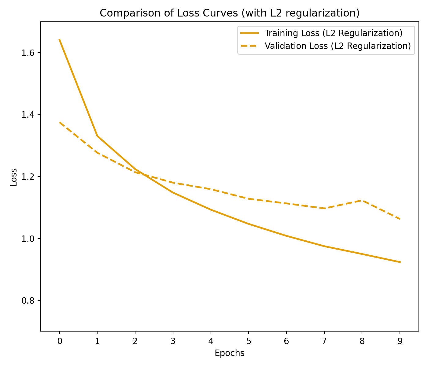Loss curves for the CNN with L2 regularization. Both, the training loss and validation loss decrease with each epoch, which is indicative of a model that is able to generalize to the validation data. Note, that the gap between the training loss and the validation loss is smaller compared to L1 regularization. This indicates that the model is able to generalize better to the validation data.

In our case, L2 regularization yields better results than L1 regularization, as the gap between the training loss and the validation loss is smaller compared to L1 regularization. This indicates that the model is able to generalize better to the validation data.

Please note that the loss curves may vary depending on the specific dataset and model architecture. The plots shown here are for illustrative purposes only and additional measures for tuning other hyperparameters may be required to achieve optimal performance.

Conclusion

L1 and L2 regularization techniques, namely Lasso and Ridge regularization, serve as powerful tools in machine learning to combat overfitting and enhance model performance. By understanding their mathematical formulations, advantages, and disadvantages, practitioners can make informed decisions when applying regularization in their models. Through the provided Python code and plots, we have demonstrated the distinct characteristics of L1 and L2 regularization, highlighting the sparsity and feature selection ability of Lasso and the stability and computational efficiency of Ridge regularization.

The code used in this post is available in this GitHub repositoryꜛ.

If you have any questions or suggestions, feel free to leave a comment below or reach out to me on Mastodonꜛ.