Information entropy
A fundamental concept that plays a pivotal role in quantifying the uncertainty or randomness of a set of data is the information entropy. Information entropy provides a measure of the average amount of information or surprise contained in a random variable. In this blog post, we explore its mathematical foundations and demonstrate its implementation in some Python examples.
Mathematical description
Let’s consider a discrete random variable $X$ with a probability mass function (PMF) given by $P(X=x)$. The information entropy $H(X)$ can be mathematically described using the following equation:
\[H(X) = -\sum_{x \in X} P(X=x) \log_{b} P(X=x)\]where $b$ represents the base of the logarithm. There are different methods to calculate $H(X)$:
Shannon entropy
Shannon entropy, proposed by Claude Shannon, is the most widely known and utilized method for calculating information entropy. It uses base 2 logarithms, resulting in entropy values measured in bits. The formula for Shannon entropy is as follows:
\[H(X) = -\sum_{x \in X} P(X=x) \log_{2} P(X=x)\]Differential entropy
Differential entropy is an extension of Shannon entropy to continuous random variables. It utilizes probability density functions (PDFs) instead of PMFs. The formula for differential entropy is given by:
\[h(X) = -\int_{-\infty}^{\infty} f(x) \log_{b} f(x) \,dx\]where $f(x)$ represents the PDF of the continuous random variable $X$.
Similarity to thermodynamic entropy
Shannon entropy has a close relationship with the concept of thermodynamic entropy discussed in the previous post. In thermodynamics, entropy is a measure of the disorder or randomness of a system. The second law of thermodynamics states that the entropy of an isolated system will always increase over time. Similarly, in information theory, information entropy measures the disorder or randomness of given discrete random variable $X$, e.g., a measured signal or a text message. The more disordered or random the $X$, the higher its entropy and the more information is needed to encode it.
Simple example
Let’s demonstrate the calculation of information entropy using Python. We will consider a simple example with a sample dataset consisting of categorical variables:
import numpy as np
import matplotlib.pyplot as plt

def calculate_entropy(pmf):
    entropy = 0
    for p in pmf:
        if p > 0:
            entropy -= p * np.log2(p)
    return entropy

# Sample dataset
data = ['A', 'B', 'A', 'C', 'B', 'A', 'A', 'C', 'B']

# Calculate PMF
pmf = np.bincount(data) / len(data)

# Calculate Shannon entropy
shannon_entropy = calculate_entropy(pmf)

# Display results
print("Shannon Entropy:", shannon_entropy)

# Plotting the PMF:
plt.figure(figsize=(4, 4))
plt.bar(range(len(pmf)), pmf)
plt.xlabel("Categories")
plt.ylabel("Probability")
plt.title("Probability Mass Function (PMF)")
plt.xticks(range(len(pmf)), categories)
plt.tight_layout()
plt.savefig("shannon_categorial_example.png", dpi=200)
plt.show()
In the provided code, we define a function calculate_entropy to compute Shannon entropy based on the probability mass function (PMF). The sample dataset $X:=\lbrace A, B, A, C, B, A, A, C, B\rbrace$ consists of categorical variables represented by letters $A$, $B$, and $C$. The PMF is calculated using np.bincount:
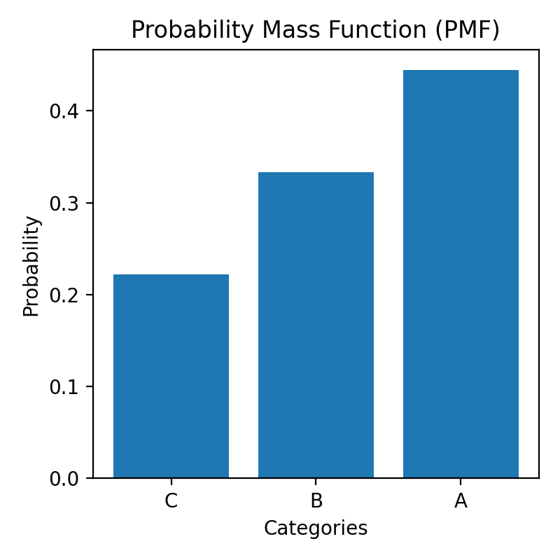 Probability Mass Function (PMF) of the sample dataset $X:=\lbrace A, B, A, C, B, A, A, C, B\rbrace$.
The resulting PMF is then used to calculate Shannon entropy, which is in our case $H(X)=1.5$ bits, which is the minimum number of bits required to encode the sample dataset.
A high entropy dataset means that the signal contains a lot of information and is less predictable. This can be desirable in certain situations, such as when transmitting sensitive information that needs to be kept secure. In this case, a high entropy dataset is harder to intercept or decode by an unauthorized party. On the other hand, a high entropy dataset can also mean that it is more difficult to compress, since it contains a lot of information. This can be a disadvantage when transmitting large amounts of data over a limited bandwidth channel.
Information rate of spike trains
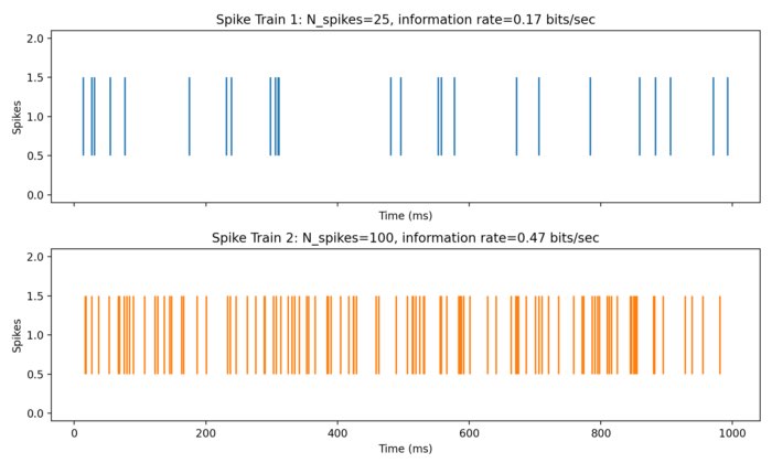
Information entropy can also be used to quantify the information rate within time series data, such as the firing rate of neurons. In neuroscience, information entropy is often used to measure the information rate of spike trains. The information rate of a spike train is defined as the amount of information contained in the spike train (i.e., the information entropy $H$) per unit time.
Here is the code for a 1000 ms simulation of two time series containing 25 and 100 random spikes, respectively:
import numpy as np
from scipy.stats import entropy
import matplotlib.pyplot as plt

# for reproducibility:
np.random.seed(0)

# simulate two spike trains for 1000 ms:
T = 1000
N_spikes_1 = 25
N_spikes_2 = 100
spike_train_1 = np.zeros(T)
spike_train_2 = np.zeros(T)
spike_times_1 = np.random.choice(T, size=N_spikes_1, replace=False)
spike_times_2 = np.random.choice(T, size=N_spikes_2, replace=False)
spike_train_1[spike_times_1] = 1
spike_train_2[spike_times_2] = 1

# calculate entropy and information rate:
counts_1 = np.bincount(spike_train_1.astype(int))
probs_1 = counts_1 / float(sum(counts_1))
H_1 = entropy(probs_1, base=2)
info_rate_1 = H_1 / (T / 1000)

counts_2 = np.bincount(spike_train_2.astype(int))
probs_2 = counts_2 / float(sum(counts_2))
H_2 = entropy(probs_2, base=2)
info_rate_2 = H_2 / (T / 1000)

# plot spike trains and information rates:
fig, axs = plt.subplots(2, 1, figsize=(10, 6), sharex=True)
axs[0].eventplot(spike_times_1, color='C0')
axs[0].set_title(f"Spike Train 1: N_spikes={N_spikes_1}, information rate={info_rate_1:.2f} bits/sec")
axs[0].set_ylabel("Spikes")
axs[0].set_xlabel("Time (ms)")
axs[1].eventplot(spike_times_2, color='C1')
axs[1].set_title(f"Spike Train 2: N_spikes={N_spikes_2}, information rate={info_rate_2:.2f} bits/sec")
axs[1].set_ylabel("Spikes")
axs[1].set_xlabel("Time (ms)")
plt.tight_layout()
plt.savefig("shannon_spike_trains.png", dpi=200)
plt.show()
 Two time series with different number of spikes, which results in different information entropies and information rates.
The plot shows that the second time series has a higher entropy and information rate than the first one. This is because series 1 has more spikes, i.e., “more information”.
Conclusion
Information entropy serves as a vital metric for quantifying uncertainty within a set of data. By understanding its mathematical foundations and employing suitable calculation methods, we gain valuable insights into the information content and randomness of various random variables, i.e., measurements. This can be useful in a wide range of applications, such as data compression, cryptography, and neuroscience.
If you have any questions or suggestions, feel free to leave a comment below or reach out to me on Mastodonꜛ.
The code used in this post is also available in this GitHub repositoryꜛ.


comments