Zarr – or: How to save NumPy arrays

Zarrꜛ is a relative young file format for storing N-dimensional arrays in Python and features:

• the creation and storing of N-dimensional NumPy arrays
• storing in memory, on disk, inside a zip file, on S3, …
• flexible chunking
• flexible compression and filtering of chunks via NumCodecs
• hierarchical organization of arrays in groups
• reading and writing arrays concurrently from multiple threads or processes

In this post we explore, how we can benefit from these features in storing and working with NumPy arrays.

Storing NumPy arrays

There are several ways to store a NumPy array on our hard drive. Common formats are human-readable textfiles (*.txt) for dimensions not higher than two and the NumPy binary file format (*.npy) with no limitation on the dimension:

import numpy as np
np.random.seed(1)
array_2D = np.random.rand(1000,1000)
array_3D = np.random.rand(1000,1000,100)

np.save("array_2D.npy", array_2D)
np.savetxt("array_2D.txt", array_2D, delimiter=" ")

np.save("array_3D.npy", array_3D)
np.savetxt("array_3D.txt", array_3D, delimiter=" ")

The last saving attempt will raise an error (ValueError: Expected 1D or 2D array, got 3D array instead) as expected, since we tried to save the 3D-array as a textfile.

While the NumPy file format seems to be the best-to-go solution for any dimensional array, they come with some limitations:

• they lack the possibility of compression, and
• they lack the possibility of parallelization of the reading and writing process.

This is where Zarr comes into play¹. Before we go into detail of its advantages, let’s first have a general look at Zarr’s read/write procedures:

import zarr
zarr_out_3D_convenient = zarr.save('zarr_out_3D_convenient.zarr', array_3D)
zarr_in_3D_convenient  = zarr.load('zarr_out_3D_convenient.zarr')
print(type(zarr_in_3D_convenient))

    <class 'numpy.ndarray'>

zarr.save()ꜛ and zarr.load()ꜛ (actually zarr.convenience.save() and zarr.convenience.load()) are Zarr’s so-called convenient functionsꜛ for saving a NumPy right away to the disk and for loading a stored Zarr array directly into the memory, respectively. For more control over the storing process we can use the creation functionꜛ zarr.creation.open()ꜛ:

zarr_out_3D = zarr.open('zarr_out_3D.zarr', mode='w', shape=array_3D.shape,
                        chunks=(1000,1000,1), dtype=array_3D.dtype)
zarr_out_3D[:] = array_3D

zarr_in_3D  = zarr.open('zarr_out_3D.zarr')

The zarr.creation.open()/zarr.open() command creates an empty Zarr file pre-allocated for the 3D NumPy array in write-mode (mode='w', create and overwrite if exists). The actual storing process is performed by the zarr_out_3D[:] = array_3D command, where the NumPy array is written to the created Zarr array. The default mode of zarr.open() is a (read/write and create if it doesn’t exist) which is why the second zarr.open() command will not overwrite the existing Zarr, but gives us access to the stored array therein and also provides the possibility to change the array entries. Please note, that the read array zarr_in_3D is not loaded into the memory unless we index or slice over all or a subset of its entries:

# this just calls some metadata about the Zarr array:
print(type(zarr_in_3D))

# this loads the entire array into the memory:
print(type(zarr_in_3D[:]))
print(zarr_in_3D.shape)

  <class 'zarr.core.Array'>
  <class 'numpy.ndarray'>
  (1000, 1000, 100)

We can work with a Zarr array as with any other NumPy array:

# e.g., calculate the mean of a subset of the array:
print(zarr_in_3D[:,:,10].mean())

# overwrite the content of that subset:
zarr_in_3D[:,:,10] = np.ones((1000,1000))
print(zarr_in_3D[:,:,10].mean())

  0.4998032068737291
  1.0

The changed entry zarr_in_3D[:,:,10] is directly written into the Zarr file as the data is automatically flushed to the file system. Therefore, there is also no need to close a Zarr array.

To add more than one array to a Zarr file, we can use the zarr.create_dataset()ꜛ command:

zarr_out_root = zarr.open('zarr_out_3Ds.zarr', mode='w')
zarr_out_3D   = zarr_out_root.create_dataset("array_3D", data=array_3D)
zarr_out_2D   = zarr_out_root.create_dataset("array_2D", data=array_2D)
print(type(zarr_out_root))
print(type(zarr_out_root["array_3D"]))
print(type(zarr_out_root["array_2D"]))

  <class 'zarr.hierarchy.Group'>
  <class 'zarr.core.Array'>
  <class 'zarr.core.Array'>

Our Zarr file has now become a hierarchical group (see below). To access a specific array in that group, simply address it by its name, e.g., zarr_out_root["array_3D"].

Attributed NumPy functions do not become available to the Zarr array unless the array is loaded into the memory via slicing or indexing:

# this will not work:
print(zarr_in_3D.mean())

# this will work:
print(zarr_in_3D[:].mean())
# and this:
numpy_in_3d = zarr_in_3D[:] 
print(numpy_in_3d.mean())

# Calling NumPy functions directly will always 
# work (will load the array into the memory as well):
print(np.mean(zarr_in_3D))

  ... AttributeError: 'Array' object has no attribute 'mean'
  0.5050569402354906
  0.5050569402354906
  0.5050569402354906

However, the Zarr array comes with some own useful attributed methods like .info, which returns a general summary of the underlying Zarr array:

print(zarr_in_3D.info)

  Type               : zarr.core.Array
  Data type          : float64
  Shape              : (1000, 1000, 100)
  Chunk shape        : (1000, 1000, 1)
  Order              : C
  Read-only          : False
  Compressor         : Blosc(cname='lz4', clevel=5, shuffle=SHUFFLE, blocksize=0)
  Store type         : zarr.storage.DirectoryStore
  No. bytes          : 800000000 (762.9M)
  No. bytes stored   : 693710592 (661.6M)
  Storage ratio      : 1.2
  Chunks initialized : 100/100

By inspecting our hard drive we may also notice, that the actual Zarr file is not a single and “closed” file. Instead, it is a folder that has the ending .zarr. Inside that folder, there is a bunch of small-sized, numerically named binary files:

ls zarr_out_3D.zarr 

  0.0.0   0.0.16  0.0.23  0.0.30  0.0.38  0.0.45  0.0.52  0.0.6   0.0.67  0.0.74  0.0.81  0.0.89  0.0.96
  0.0.1   0.0.17  0.0.24  0.0.31  0.0.39  0.0.46  0.0.53  0.0.60  0.0.68  0.0.75  0.0.82  0.0.9   0.0.97
  0.0.10  0.0.18  0.0.25  0.0.32  0.0.4   0.0.47  0.0.54  0.0.61  0.0.69  0.0.76  0.0.83  0.0.90  0.0.98
  0.0.11  0.0.19  0.0.26  0.0.33  0.0.40  0.0.48  0.0.55  0.0.62  0.0.7   0.0.77  0.0.84  0.0.91  0.0.99
  0.0.12  0.0.2   0.0.27  0.0.34  0.0.41  0.0.49  0.0.56  0.0.63  0.0.70  0.0.78  0.0.85  0.0.92
  0.0.13  0.0.20  0.0.28  0.0.35  0.0.42  0.0.5   0.0.57  0.0.64  0.0.71  0.0.79  0.0.86  0.0.93
  0.0.14  0.0.21  0.0.29  0.0.36  0.0.43  0.0.50  0.0.58  0.0.65  0.0.72  0.0.8   0.0.87  0.0.94
  0.0.15  0.0.22  0.0.3   0.0.37  0.0.44  0.0.51  0.0.59  0.0.66  0.0.73  0.0.80  0.0.88  0.0.95

It’s 100 files in total,

ls zarr_out_3D.zarr | wc -l

  100

and this number is no coincidence – it corresponds exactly to the chunk size that we set when we created the Zarr array. We set the size of a single chunk to chunks=(1000,1000,1), which results for a given array shape of (1000, 1000, 100) to 100 chunks. So, each of these 100 files corresponds exactly to one chunk of the array. You can cross-check this by setting the chunk size to (1000,1000,100),

zarr_out_3D_one_chunk = zarr.open('zarr_out_3D_one_big_chunk.zarr', mode='w', shape=array_3D.shape,
                        chunks=(1000,1000,100), dtype=array_3D.dtype)
zarr_out_3D_one_chunk[:] = array_3D

and you get one big chunk that contains the entire array:

ls zarr_out_3D_one_big_chunk.zarr 

    0.0.0

But what are chunks good for?

Memory mapping and chunking

Before we go deeper into chunking, let’s first have a look at the OS’ general read/write procedure. Normally, when a file is loaded from disk, it is first copied into the OS’ memory (“buffer cache”) and then passed to the programm’s memory²:

While the communication between the disk and the buffer cache is relatively slow and depends on the performance of the hard drive, the communication between the buffer cache and the program memory is orders of magnitude faster. The buffer cache is therefore kept to provide a fast reaccessing of the data to the program memory:

But in case the memory is needed for something else, the OS will clear the cache.

Writing data back to disk works in the same way, just in the opposite direction. Again, since the communication between the buffer cache and the program memory is quite fast, writing is also usually quick. It is first written to the cache (fast) and then flushed to the disk (slow). For the latter step, the program no longer has to wait for and can continue its further processing:

As long as the data fits into the buffer cache, reading and writing works quite fast. But when the data becomes too large, we run into trouble, either regarding read/write speeds or being able to load the data into the memory at all. And for such situations there are two strategies that address this problem:

• memory mapping, and
• chunking

With memory mapping, an array is saved into one file on the disk. When reading and writing to it, the entire file is treated by the OS “transparently”, i.e., it is just treated as if it were completely in the memory. The file is mapped to a range of addresses within the program’s address space (emulating the actual buffer cache inside the program’s memory), and the program can access the content of the file in the same way as it would access content from the memory³:

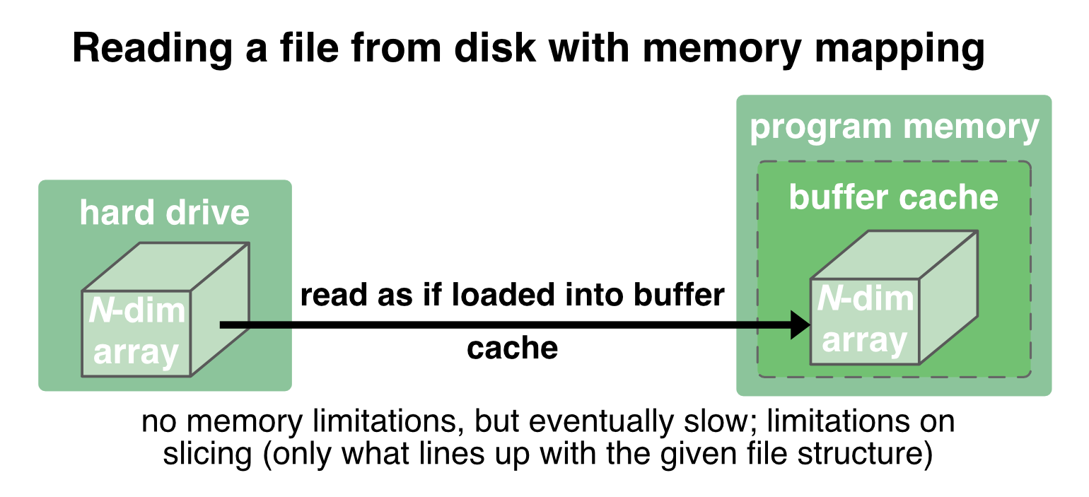
If parts of the data is already loaded into the actual memory, the OS reads/writes these parts directly into the program memory (which is fast), otherwise it transparently (but slower) reads/writes it from disk into the program memory.

To perform memory mapping of an array in Python is quite easy, as NumPy brings its own memory mapping function mmap()ꜛ:

# create an empty memory mapped file:
numpy_mmap_3D = np.memmap("numpy_out_3D.arr", mode="w+", dtype=array_3D.dtype, 
                          shape=array_3D.shape)

# write the array to that file:
numpy_mmap_3D[:] = array_3D

# and flush to disk:
numpy_mmap_3D.flush()

# reaccess the array via:
numpy_mmap_3D_read = np.memmap("numpy_out_3D.arr", mode="r", dtype=array_3D.dtype, 
                               shape=array_3D.shape)
print(np.array_equal(array_3D, numpy_mmap_3D_read))

    True

mmap() works very well for many use cases. However, it also has some draw-backs:

• Slicing is restricted to the given structure within the memory mapped file. If we want to slice a stored array along axes that do not follow the given structure within the file, reading and writing will become slow as it requires large numbers of disk reads.
• If the file parts, that are already buffered in the memory, exceed the capacity of the memory, the OS will indeed transparently load additionally requested file parts from disk, but this is much slower than reading directly from the actual memory.
• The data needs to be stored on the local file system.

Zarr¹ files overcome these disadvantages by storing and loading the array in chunks. With chunking, an array is stored to the disk into several small bits. These bits are loaded into the memory only when they are requested/called, e.g., to perform a specific operation just on that chunks:

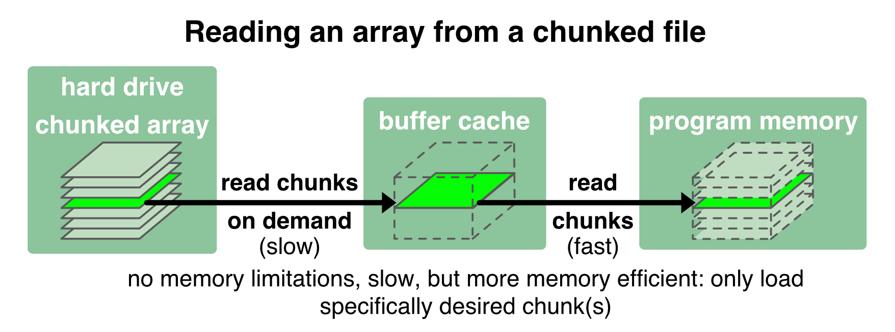
With Zarr we have full control over the file’s chunk size. We have already set an individual chunk size when we created the second Zarr file in the example above (zarr_out_3D.zarr). When our program requests a specific chunk from the Zarr file (i.e., “slicing” the array), only that chunk is loaded into the buffer cache. In the same way, the changed content of a read chunk is written back to the chunked file.

Chunks and parallelization

A reasonable chunking also enables an efficient parallelization of the array processing. For instance, in case it is necessary to process a 3D array along a certain axis (e.g., for median-filtering a 3D image slice-by-slice), we can chunk that array accordingly, so that in a parallelized processing only the currently required slices are efficiently loaded into the memory and written back to the file after the processing.

Compression

Another advantage of Zarr files¹ is, that chunks can be additionally compressed. Why is this a good thing? The chunked and compressed content of a file can be loaded much faster than the actual bandwidth of the hard drive. For instance, with the compression ratio of 1.2 in our example from above (Storage ratio: 1.2) the chunks are loaded 1.2 times faster than the disk bandwidth minus the time it takes to decompress the chunks:

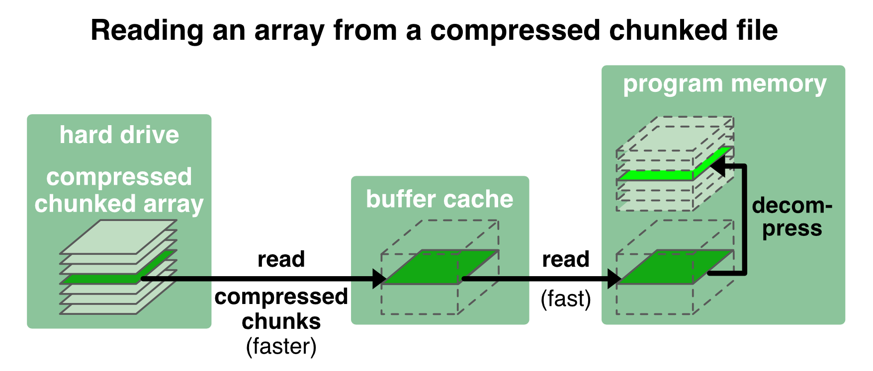
Zarr offers several compressors via the NumCodecsꜛ package. The .info call in the example from above reveals, that Zarr already applies some compression by default (Blosc(cname='lz4', clevel=5, shuffle=SHUFFLE, blocksize=0)). We can further specify the compression, e.g., when creating the Zarr file:

from numcodecs import Blosc
compressor  = Blosc(cname='zstd', clevel=5, shuffle=Blosc.BITSHUFFLE)
zarr_out_3D = zarr.open('zarr_out_3D_compressed.zarr', mode='w', shape=array_3D.shape,
                        chunks=(1000,1000,1), dtype=array_3D.dtype, compressor=compressor)
zarr_out_3D[:] = array_3D
print(zarr_out_3D.info)

  Type               : zarr.core.Array
  Data type          : float64
  Shape              : (1000, 1000, 100)
  Chunk shape        : (1000, 1000, 1)
  Order              : C
  Read-only          : False
  Compressor         : Blosc(cname='zstd', clevel=5, shuffle=BITSHUFFLE, blocksize=0)
  Store type         : zarr.storage.DirectoryStore
  No. bytes          : 800000000 (762.9M)
  No. bytes stored   : 688243152 (656.4M)
  Storage ratio      : 1.2
  Chunks initialized : 100/100

Please note, that floating point numbers are less compressible than integer numbers:

array_3D_int    = np.random.randint(low=1, high=10, size=(1000,1000,100), dtype="int64")
compressor      = Blosc(cname='zstd', clevel=5, shuffle=Blosc.BITSHUFFLE)
zarr_out_3D_int = zarr.open('zarr_out_3D_compressed_int.zarr', mode='w', shape=array_3D_int.shape,
                        chunks=(1000,1000,1), dtype=array_3D_int.dtype, compressor=compressor)
zarr_out_3D_int[:] = array_3D_int
print(zarr_out_3D_int.info)

  Type               : zarr.core.Array
  Data type          : int64
  Shape              : (1000, 1000, 100)
  Chunk shape        : (1000, 1000, 1)
  Order              : C
  Read-only          : False
  Compressor         : Blosc(cname='zstd', clevel=5, shuffle=BITSHUFFLE, blocksize=0)
  Store type         : zarr.storage.DirectoryStore
  No. bytes          : 800000000 (762.9M)
  No. bytes stored   : 49050950 (46.8M)
  Storage ratio      : 16.3
  Chunks initialized : 100/100

Groups

Zarr also supports the hierarchical organization of arrays, which means, that we can store more than one array in a Zarr file and arrange these arrays in a hierarchical manner. This is done via so-called groupsꜛ:

# create a new Zarr file
zarr_out_root = zarr.open('zarr_out_3D.zarr', mode='w')

# store two different arrays to the root of the Zarr file:
zarr_out_3D   = zarr_out_root.create_dataset("array_3D", data=array_3D)
zarr_out_2D   = zarr_out_root.create_dataset("array_2D", data=array_2D)

# create a first group and add an array to it:
zarr_out_root.create_group("group_1")
zarr_out_root["group_1"].create_dataset("array_1D_1",data=np.arange(1000))

# create another group and add some arrays in one command:
zarr_out_sub_1D_1 = zarr_out_root.create_dataset("group_2/array_1D_2", data=np.arange(100))
zarr_out_sub_1D_2 = zarr_out_root.create_dataset("group_2/array_1D_3", data=np.arange(10))

# inspect the created hierarchy:
print(zarr_out_root.tree())

  /
   ├── array_2D (1000, 1000) float64
   ├── array_3D (1000, 1000, 100) float64
   ├── group_1
   │   └── array_1D_1 (1000,) int64
   └── group_2
       ├── array_1D_2 (100,) int64
       └── array_1D_3 (10,) int64

There are several ways to access an array from a specific group:

zarr_in_root = zarr.open('zarr_out_3D.zarr', mode='r')
zarr_in_group_1 = zarr_in_root["group_1/array_1D_1"]

# or:
zarr_in_group_1 = zarr.open('zarr_out_3D.zarr/group_1/array_1D_1', mode='r')

Arrays that are organized in groups can be accessed and manipulated like any other array stored in the Zarr file.

Attributes

Another quite useful feature of Zarr are attributes. They can be assigned to the root file as well as to the arrays and groups therein. They can serve as custom user-metadata:

# assign attributes to the (root) Zarr file:
zarr_out_root.attrs["author"] = "Pixel Tracker"
zarr_out_root.attrs["date"]   = "Oct 13, 2022"
zarr_out_root.attrs["description"]  = "A Zarr file containing some NumPy arrays"

# assign attributes to groups:
zarr_out_root["group_1"].attrs["description"] = "A test sub-group"

# assign attributes to arrays:
zarr_out_root["group_1/array_1D_1"].attrs["description"] = "A test array"

# list attributes:
for key in zarr_out_root.attrs.keys():
    print(f"{key}: {zarr_out_root.attrs[key]}")
print(zarr_out_root["group_1"].attrs["description"])
print(zarr_out_root["group_1/array_1D_1"].attrs["description"])

  author: Pixel Tracker
  date: Oct 13, 2022
  description: A Zarr file containing some NumPy arrays
  A test sub-group
  A test array

Attributes as well as the general info about the Zarr arrays is stored within the Zarr file in a human-readable format (JSON):

cat zarr_out_3D.zarr/.zattrs 

  {
      "author": "Pixel Tracker",
      "date": "Oct 13, 2022",
      "description": "A Zarr file containing some NumPy arrays"
  }

cat zarr_out_3D.zarr/array_3D/.zarray 

  {
      "chunks": [
          125,
          125,
          13
      ],
      "compressor": {
          "blocksize": 0,
          "clevel": 5,
          "cname": "lz4",
          "id": "blosc",
          "shuffle": 1
      },
      "dtype": "<f8",
      "fill_value": 0.0,
      "filters": null,
      "order": "C",
      "shape": [
          1000,
          1000,
          100
      ],
      "zarr_format": 2
  }

You can open these .zarray and .zattrs files also with the default text editor of your OS and view basic information about the underlying Zarr file, without running any Python code.

Accessing Zarr arrays from the cloud

The access to Zarr arrays is not limited to the local file system or local network. It is also possible to store and read Zarr files from distributed (cloud) storages like Amazon’s Simple Storage Service S3 (S3Fs), the Hadoop Distributed File System (HDFSMapꜛ), Google Cloud Storage (GCSMapꜛ) and Microsoft’s Azure Blob Storage (ABSStoreꜛ). The good thing here is, that the Zarr arrays stored in the cloud are treated during our local processing as if they were stored on the local file system. Here is an example for a Zarr array stored in the public S3 bucket eu-west-2:

import s3fs
s3_fs     = s3fs.S3FileSystem(anon=True, client_kwargs=dict(region_name='eu-west-2'))
s3_store  = s3fs.S3Map(root='zarr-demo/store', s3=s3_fs, check=False)
zarr_root = zarr.group(store=s3_store)
z_array   = zarr_root['foo/bar/baz']
print(z_array)
print(z_array.info)
print(z_array[:].tobytes())

  <zarr.core.Array '/foo/bar/baz' (21,) |S1>
  Name               : /foo/bar/baz
  Type               : zarr.core.Array
  Data type          : |S1
  Shape              : (21,)
  Chunk shape        : (7,)
  Order              : C
  Read-only          : False
  Compressor         : Blosc(cname='lz4', clevel=5, shuffle=SHUFFLE, blocksize=0)
  Store type         : zarr.storage.KVStore
  No. bytes          : 21
  No. bytes stored   : 382
  Storage ratio      : 0.1
  Chunks initialized : 3/3
  
  b'Hello from the cloud!'

Reading and writing from and to the cloud introduces of course an additional bottleneck due to the network speed. The Zarr documentationꜛ provides some hacks how to speed this up a little.

Conclusion

With Zarr we do not only have another file format for storing NumPy arrays. It allows the organization of multiple arrays within one file directory. We could even think of managing parts or even an entire (small) project within one Zarr file. Furthermore, Zarr provides an efficient solution for handling big arrays, that do not fit into the memory. The customizability of the chunk size and compressors allows the implementation of efficient parallelization strategies for processing multidimensional arrays. And with its support for distributed storages we can easily treat Zarr arrays stored in the cloud just like any other array stored on our local file system.

Even though it’s a quite young file format, overcoming the limitations of NumPy and HDF5¹ files, I have the impression that it is becoming more and more popular and used. Nowadays it is already ported or in development of porting to other programming languages like Juliaꜛ, C++ꜛ, Javaꜛ, or Rꜛ. I started to use Zarr in almost all my image processing pipelines.

Have you already worked with it Zarr? Or do you have ideas for its application? Please feel free to share your thoughts in the comment section below.

The Python code used in this post is also available in this GitHub repositoryꜛ.

Footnotes

1. The disadvantages of the NumPy file format can also be overcome by using the HDF5 file format, which is fairly similar to Zarr. In this post I will focus on Zarr only. If you’re interested in a detailed comparison between Zarr and HDF5, watch this in-depth presentationꜛ by Joe Jevnik or this presentationꜛ by Alistair Milesꜛ. ↩ ↩² ↩³ ↩⁴

2. The illustrations on memory mapping are adapted from pythonspeed.com. ↩

3. Cited after askpython.com. ↩