Chapter 10: NumPy - Our data container

The evaluation of scientific data, i.e. measurement data, is almost always about the evaluation of numbers. This applies, e.g., to LFP time series, patch-clamp recordings or multi-fluorescence images.

The mathematical functions of pure Python are limited. Anything beyond basic operations (+, -, /, *) has to be programmed by ourselves. We can of course do that – or: We use one of the many packages where others have already done the work for us. Such a useful package is NumPy (numpy.org/doc/stable/).

The NumPy logo. Image source: commons.wikimedia.org, license: CC BY-SA 4.0

Introduction

Let’s have a first look:

import numpy as np

# let's create our first NumPy-array:
array_1 = np.arange(10)
array_2 = np.array([1, 2, 3])
print(f"array_1: {array_1}")
print(f"array_2: {array_2}")

array_1: [0 1 2 3 4 5 6 7 8 9]
array_2: [1 2 3]

The import command makes all functions within the NumPy package available for our own program. These functions can be called by np.FUNCTION(...), e.g. np.mean(array_1):

print(f"np.mean(array_1): {np.mean(array_1)}")

np.mean(array_1): 4.5

The np.arange(start,stop,step) command creates a so-called NumPy-array similar to the range command, but with the advantage that we can directly access the array (to achieve the same with the range command: list(range(10))). And we now can create arrays with floating point numbers:

array_3 = np.arange(0, 5, 0.5)
print(f"array_1: {array_3}")

array_1: [0. 0.5 1. 1.5 2. 2.5 3. 3.5 4. 4.5]

The np.array([1, 2, 3]) command converts any given list (or other array-like object) into a NumPy array.

One main advantage of a NumPy array is, that one can directly call basic NumPy functions via array.mean() instead of np.mean(array) (while both is valid):

print(f"array_1.mean(): {array_1.mean()}")

array_1.mean(): 4.5

Some further examples:

print(f"array_1.std(): {array_1.std()}")
print(f"array_1.max(): {array_1.max()}")
print(f"array_1.min(): {array_1.min()}")
print(f"array_1.sum(): {array_1.sum()}")

array_1.std(): 2.8722813232690143
array_1.max(): 9
array_1.min(): 0
array_1.sum(): 45

Not all NumPy functions can be accessed this way:

print(f"array_1.median(): {array_1.median()}")

AttributeError...

print(f"np.median(array_1): {np.median(array_1)}")

np.median(array_1): 4.5

Useful NumPy functions

Command	Description
Creating and manipulating arrays:
np.arange(number)	creates an array of evenly spaced values, e.g. np.arange(3) creates an array of the numbers 1, 2, 3
np.array([1,2,3])	creates an array, e.g., of the numbers 1, 2, 3
np.shape(array)	get the shape (dimensions and lengths) of array
array.dtype	get the type of array (integer?, float?, …)
array.reshape	reshapes array, e.g. from shape (6) to (2,3)
np.transpose or array.T	transpose array
np.append(array1, array2)	append array1 to array2
np.concatenate((array1, array2))	concatenate array1 and array2
np.insert(array, index, value)	insert value at index-position of array
np.delete(array, index)	delete entry at index-position of array
Useful statistical functions:
np.mean(array)	calculate the average of array
np.median(array)	calculate the median of array
np.std(array)	calculate the standard deviation of array
np.sum(array)	calculate the sum of array
np.cumsum(array)	calculate the cumulative sum of array
np.max(array)	calculate the maximum of array
np.min(array)	calculate the minimum of array
Useful mathematical functions:
np.sqrt(array)	calculate the square root of array
np.square(array)	calculate the square of array
np.abs(array)	calculate the element-wise absolute values of array
np.exp(array)	calculate the exponentiation of array
np.log(array)	calculate the natural logarithm of array
np.sin(array)	calculate the sine of array
np.cos(array)	calculate the cosine of array
np.round(array)	round array
np.floor(array)	floor of the array
np.ceil(array)	ceiling of the array
np.sort(array)	sort array
np.nan_to_num(array)	replace NaN (Not a Number) with zero and infinity with large finite numberization

You can find a broader overview of NumPy functions, e.g., on the Datacamp ꜛ NumPy cheat sheet ꜛ.

Of course, you can also construct your own functions using existing NumPy functions, e.g.:

""" Let's construct a simple function, that searches the closest 
    value within an NumPy for a given search value: 
"""
import numpy as np

# define the function:
def find_nearest(input_array, search_number):
    """
    Simple function to search for the closest
    value within a given NumPy array.
    
    input_array:   input array within we search
    search_number: integer or floating point 
                   number to search for in
                   input_array
                   
    Caution: This function is not bullet-proof: It does 
    not return multiple occurrences of the found 
    closest(s) value(s).
    """
    array = np.asarray(input_array)
    idx = (np.abs(array - search_number)).argmin()
    return array[idx], idx

# apply the function to a test array:
array_test = np.array([0, 5, 5, 6, 6, 3, 9])
print(array_test)
print(find_nearest(array_test, 5.6))

[0, 5, 5, 6, 6, 3, 9]
6, 3

On array dimensionality

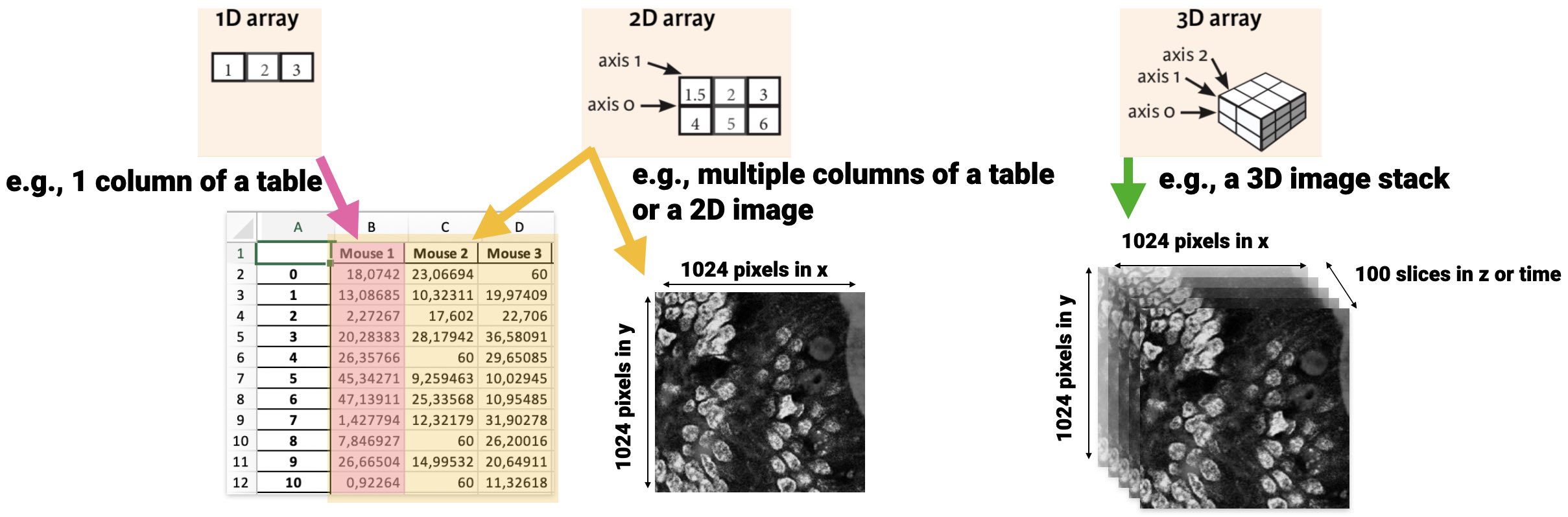
One very useful NumPy command is np.shape(array) or array.shape, which returns the size and the shape (dimensions) of a given array:

print(f"array_1.shape(): {array_1.shape}")

array_1.shape(): (10,)

The output (10,) indicated, that array_1 has only one axis, i.e. it is one-dimensional, with 10 entries on that axis. We can of course create NumPy arrays with higher dimensions:

# 2D array (e.g. an image):
array_4 = np.array([(1, 2, 3),    
                    (4, 5, 6),
                    (7, 8, 9),
                    (7, 8, 9)])
print(f"array_4:")
print(array_4)
print(f"array_4.shape(): {array_4.shape}")

array_4:
[[1 2 3]
[4 5 6]
[7 8 9]
[7 8 9]]
array_4.shape(): (4, 3)

# 3D array (e.g. an image stack):
array_5 = np.array([[(1,2,3), (4,5,6)],
                    [(3,2,1), (4,5,6)]])
print(f"array_5:")
print(array_5)
print(f"array_5.shape(): {array_5.shape}")

array_5:
[[[1 2 3]
[4 5 6]] [[3 2 1]
[4 5 6]]]
array_5.shape(): (2, 2, 3)

Visual overview of NumPy array dimensionalities:

Multi-fluorescence image source: commons.wikimedia.org, license: CC BY 2.0; array dimension sketches taken from the Datacamp ꜛ NumPy cheat sheet. ꜛ

Useful helper functions for array generation

NumPy brings some little helper functions to create $n$-dimensional arrays (sometimes helpful in prototyping and testing your programs or to understand a program):

# let NumPy create some arrays:
Z = np.zeros((3,4))
print(f"Z:")
print(Z)

Z:
[[0. 0. 0. 0.]
[0. 0. 0. 0.]
[0. 0. 0. 0.]]

O = np.ones((3,4))
print(f"O:")
print(O)

O:
[[1. 1. 1. 1.]
[1. 1. 1. 1.]
[1. 1. 1. 1.]]

L = np.linspace((1,21),(5,25),5)
""" creates a 2D array; 1st column ranges from 1 (of (1,11))
    to 5 (of (5,15)), automatically spaced, so that we get
    5 (last number in the command) equally spaced increasing
    numbers. """
print(f"L:")
print(L)

L:
[[ 1. 21.]
[ 2. 22.]
[ 3. 23.]
[ 4. 24.]
[ 5. 25.]]

np.random.seed(1)
R = np.random.random((4,3))
# Creates some random numbers. The command np.random.seed(1)
#  fixes the machine internal random state for reproducibility.
print(f"R:")
print(R)

R:
[[4.17022005e-01 7.20324493e-01 1.14374817e-04]
[3.02332573e-01 1.46755891e-01 9.23385948e-02]
[1.86260211e-01 3.45560727e-01 3.96767474e-01]
[5.38816734e-01 4.19194514e-01 6.85219500e-01]]

Indexing and slicing

Indexing and slicing of NumPy arrays works similar as for lists:

print(f"shape of R: {R.shape} (4 rows, 3 columns)")

shape of R: (4, 3) (4 rows, 3 columns)

print(f"R[0,0]:")
print(R[0,0]) # Note, R is 2D and needs therefore two
              #    index-values:
              #    first: row-index, second: column-index

R[0,0]:
0.417022004702574

print(f"R[:,0]:")
print(R[:,0])

R[:,0]:
[0.417022 0.30233257 0.18626021 0.53881673]

print(f"R[1:4,0]:")
print(R[1:4,0])

R[1:4,0]:
[0.30233257 0.18626021 0.53881673]

Also the output of the shape command is indexable:

print(f"R.shape[0]: {R.shape[0]} (4 rows)")
print(f"R.shape[1]: {R.shape[1]} (3 columns)")

R.shape[0]: 4 (4 rows)
R.shape[1]: 3 (3 columns)

Exercise 1

Write a script, that defines the 2D NumPy array L as defined above/as follows:

L = np.linspace((1,11),
                (5,15),
                 5)

Iterate L

• over each row. Calculate and print the average of each row.
• over each column. Calculate and print the average of each column.

# Your solution here:

L:
[[ 1. 21.]
[ 2. 22.]
[ 3. 23.]
[ 4. 24.]
[ 5. 25.]]
averages over rows:
11.0
12.0
13.0
14.0
15.0
averages over columns:
3.0
23.0

Toggle solution

# Solution 1:
print("L:")
print(L)

print("averages over rows:")
for row in range(L.shape[0]):
    print(L[row,:].mean())

print("averages over columns:")
for column in range(L.shape[1]):
    print(L[:,column].mean())

# just a test to create, e.g., a 3x5 Matrix:
L = np.linspace((1,11, 7),
                (5,15, 11),
                 9)
print(L)

[[ 1. 11. 7. ]
[ 1.5 11.5 7.5]
[ 2. 12. 8. ]
[ 2.5 12.5 8.5]
[ 3. 13. 9. ]
[ 3.5 13.5 9.5]
[ 4. 14. 10. ]
[ 4.5 14.5 10.5]
[ 5. 15. 11. ]]

# just a test to create a one-line vector:
L = np.linspace(1, 5, 9) # 1=start, 5=stop, 9=number of steps
print(L)

[1. 1.5 2. 2.5 3. 3.5 4. 4.5 5. ]

Exercise 2

Given the NumPy array A, that is defined as follows:

A = np.array([np.arange(0,3,1)]*5,dtype='float16')

Write a script that

1. prints out its shape.
2. prints out all entries of column 1 and 2, separately and at once.
3. overwrites the values of column 1 by the sum of the values of columns 2 and 3.
4. replaces the entry of row 1, column 3 with its exponentiation with the factor 2 (Hint: x**2).
5. replaces the entry of row 2, column 3 with the square root (np.sqrt(value)) of the entry of row 2, column 0 .
6. prints out all entries with even index values of column 3.
7. calculates the average and standard deviation of all entries of column 3.

# Your solution 2.1 here:

A:
[[0. 1. 2.]
[0. 1. 2.]
[0. 1. 2.]
[0. 1. 2.]
[0. 1. 2.]]
A.shape: (5, 3)

Toggle solution

# Solution 2.1:
A = np.array([np.arange(0,3,1)]*5,dtype='float16')
print("A:")
print(A)
print(f"A.shape: {A.shape}")

# Your solution 2.2 here:

[0. 0. 0. 0. 0.] [1. 1. 1. 1. 1.] [[0. 1.] [0. 1.] [0. 1.] [0. 1.] [0. 1.]]

Toggle solution

# Solution 2.2:
print(A[:, 0])
print(A[:, 1])
print(A[:, 0:2])

# Your solution 2.3 here:

[[3. 1. 2.]
[3. 1. 2.]
[3. 1. 2.]
[3. 1. 2.]
[3. 1. 2.]]

Toggle solution

# Solution 2.3:
A[:,0] = A[:,1] + A[:,2]
print(A)

# Your solution 2.4 and 2.5 here:

4.0
1.732
[[3. 1. 4. ]
[3. 1. 1.732]
[3. 1. 2. ]
[3. 1. 2. ]
[3. 1. 2. ]]

Toggle solution

# Solution 2.4 and 2.5:
A[0,2] = A[0,2]**2
A[1,2] = np.sqrt(A[1,0])
print(A[0,2])
print(A[1,2])
print(A)

# Your solution 2.6 here:

[4. 2. 2.]

Toggle solution

# Solution 2.6:
print(A[0:5:2, 2]) # all entries with even index of column 3

# Your solution 2.7 here:

the result: 2.345703125 +/- 0.83349609375

Toggle solution

# Solution 2.7:
print(f"the result: {A[:,2].mean()} +/- {A[:,2].std()}")

# we can also round the numbers (unfortunately, my
#  Jupyter Notebook produces some error here; in your
#  Spyder Editor it should work correctly)
#  e.g. round(2.65789, 2) means: round the 2.65789 to a
#       number with 2 floating point numbers (here to: 2.66)
print(f"{round(A[:,2].mean(), 2)} +/- {round(A[:,2].std(),2)}")

2.349609375 +/- 0.830078125

Exercise 3

1. Generate a Numpy array time ranging from 0 to 5 in steps of 0.1.
2. Calculate the exponential values \(y = e^{time}\) (Hint: np.exp(array)).
3. Copy your created y into another variable called, e.g., y_noisy.
4. Add some noise to y_noisy by adding np.random.randn(len(time))*10.
5. Import the Gaussian 1D filter function from the scipy ndimage package:

   from scipy.ndimage import gaussian_filter1d
   

   If the scipy module is missing, please install it. Please inform yourself about this function on docs.scipy.org ꜛ.

6. Apply the Gaussian filter to the noisy signal (gaussian_filter1d(y_noisy, sigma))
   1. with sigma = 3
   2. with sigma = 6

(again, save your results into new variables, e.g., y_denoised_3 and y_denoised_6)

# Your solution here:

Toggle solution

# Solution 3:
import numpy as np
from scipy.ndimage import gaussian_filter1d

# create data arrays:
time = np.arange(0,5, 0.1)
y = np.exp(time)

# add some noise:
y_noisy = y.copy()
y_noisy = y_noisy  + np.random.randn(len(time))*10

# apply filters:
y_denoised_3 = gaussian_filter1d(y_noisy, 3)
y_denoised_6 = gaussian_filter1d(y_noisy, 6)

Shallow vs. Deep Copy

Also for NumPy arrays account the shallow and deep copy rules we have learned before:

# shallow copy only:
array_1 = np.arange(0,3,1)  # create the first array_1
array_2 = array_1           # create another array by
                            # shallow copying array_1
print("array_2 after shallow copying array_1:")
print("array_1:", array_1, "array_2:", array_2)

array_2 after shallow copying array_1:
array_1: [0 1 2] array_2: [0 1 2]

# modify the shallow copy:
array_2[1] = -7

print("array_2 modified after shallow copying array_1:")
print('array_1:', array_1, 'array_2:', array_2)

array_2 modified after shallow copying array_1:
array_1: [ 0 -7 2] array_2: [ 0 -7 2]

Note, that also array_1 has been modified, too!

# deep copy:
array_2 = array_1.copy()  # deep copy in NumPy
array_2[1] = 20

print("array_2 modified after deep copying array_1:")
print('array_1:', array_1, 'array_2:', array_2)

array_2 modified after deep copying array_1:
array_1: [ 0 -7 2] array_2: [ 0 20 2]

A deep copy with NumPy can be achieved via the following commands:

• array.copy()
• np.copy(array)