The Lotka-Volterra equations: Modeling predator-prey dynamics
The Lotka-Volterra equations, also known as the predator-prey equations, is a mathematical model that describes the interaction between two species: predators and their prey. It was independently developed by Alfred J. Lotka and Vito Volterra in the early 20th century. The system captures the dynamic relationship between the population sizes of predators and prey over time, highlighting the intricate balance between them. In this post we explore this system and calculate its numerical solution using numerical integration Python.
The mathematical model
The system is defined by the following variables:
- $x(t)$: The number of prey at time $t$.
- $y(t)$: The number of predators at time $t$.
- $a$: Reproduction rate of prey.
- $b$: Predator feeding rate per prey creature (prey mortality rate per predator).
- $c$: Predator mortality rate when prey is not available.
- $d$: Reproduction rate of predators per prey species.
The Lotka-Volterra system consists of two coupled first-order ordinary differential equations:
\[\begin{align*} \frac{dx}{dt} &= a \cdot x - b \cdot x \cdot y \\ \frac{dy}{dt} &= c \cdot x \cdot y - d \cdot y \end{align*}\]The first equation represents the rate of change of the prey population over time. It takes into account the reproduction of prey at a rate proportional to their population size, as well as the decrease in prey population due to predation.
The second equation describes the rate of change of the predator population. It considers the increase in predators due to successful hunting and feeding on prey, as well as the decrease in predators due to natural mortality.
The Lotka-Volterra system exhibits interesting dynamics that emerge from the interaction between predators and prey. By solving the differential equations numerically, we can visualize the population trajectories and gain insights into the behavior of the system.
Solving and plotting the Lotka-Volterra equations
Let’s now use Python code to solve and plot the Lotka-Volterra system. We’ll employ the solve_ivp function from the scipy.integrate module to numerically solve the system of equations.
For reproducibility:
conda create -n lotkavolterra -y python=3.8
conda activate lotkavolterra
conda install -y numpy matplotlib scikit-learn ipykernel
Here’s the code:
# %% IMPORTS
import numpy as np
from scipy.integrate import solve_ivp
import matplotlib.pyplot as plt

# %% Lotka-Volterra equations:
def lotkavolterra(t, z, a, b, c, d):
    x, y = z
    return [a * x - b * x * y, c * x * y - d * y]

a = 0.4   # Reproduction rate of prey
b = 0.001   # Predator feeding rate per prey creature
c = 0.003   # Predator mortality rate when prey is not available
d = 0.6   # Reproduction rate of predators per prey species

x0 = 600   # Initial population of the prey
y0 = 500    # Initial population of the predator
time_span = [0, 50] # in years

sol = solve_ivp(lotkavolterra, time_span, [x0, y0], args=(a, b, c, d), dense_output=True)

t = np.linspace(0, time_span[1], 300)
y_Sol = sol.sol(t)

# Plotting population dynamics
fig = plt.figure(figsize=(6, 4))
plt.plot(t, y_Sol[0,].T, alpha=1, lw=2, label='prey')
plt.plot(t, y_Sol[1,].T, alpha=1, lw=2, label='predator')
plt.xlabel('time')
plt.ylabel('population')
plt.title('Lotka-Volterra System')
plt.ylim(0, 2000)
plt.legend()
plt.tight_layout()
plt.savefig('Lotka_Volterra_System.png', dpi=200)
plt.show()

# Plotting phase space
fig = plt.figure(figsize=(6, 4))
plt.plot(y_Sol[0,:], y_Sol[1,:], alpha=1, lw=2)
plt.xlabel('Population of prey')
plt.ylabel('Population of predators')
plt.title('Lotka-Volterra System (phase space)')
plt.xlim(0, 1000)
plt.ylim(0, 2000)
plt.legend()
plt.tight_layout()
plt.savefig('Lotka_Volterra_System_phase_space.png', dpi=200)
plt.show()
In the code above, we define the lotkavolterra function to represent the differential equations of the Lotka-Volterra system. We then set the parameter values and initial populations. By using solve_ivp, we obtain the numerical solution sol over the specified time span.
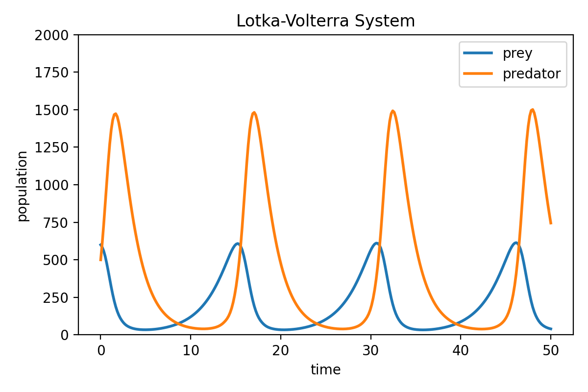
The first plot shows the population dynamics of prey and predators over time. The prey population exhibits cyclic behavior, with oscillations corresponding to the interaction with the predator population. The predator population, on the other hand, responds to changes in prey availability, resulting in periodic fluctuations as well.
 Solution of the Lotka-Volterra system. The prey population exhibits cyclic behavior, with oscillations corresponding to the interaction with the predator population. The predator population, on the other hand, responds to changes in prey availability, resulting in periodic fluctuations as well.
The second plot depicts the phase space of the system, illustrating the relationship between the population sizes of prey and predators. The trajectory forms closed loops, indicating the cyclical nature of the system.
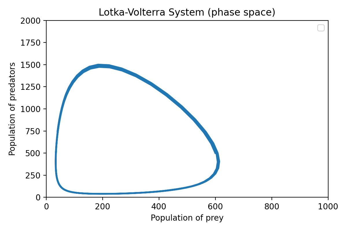 Phase space representation of the Lotka-Volterra system. The trajectory forms closed loops, indicating the cyclical nature of the system.
Feel free to modify the parameter values and initial populations to explore the dynamics of the system.
Conclusion
The Lotka-Volterra system provides a valuable framework for studying predator-prey dynamics. By mathematically modeling the interactions between species, we can gain insights into the complex and often delicate relationships that exist in ecosystems. The system’s ability to generate oscillatory behavior and cyclical population dynamics makes it an intriguing and useful tool in ecology, biology, and other fields.
There are further variations and extensions of the Lotka-Volterra system that incorporate additional factors, such as the carrying capacity of the environment and the effects of environmental fluctuations. These extensions can be used to model more complex ecological systems and investigate the effects of environmental changes on predator-prey dynamics.
The code used in this post is available in this GitHub repositoryꜛ.
If you have any questions or suggestions, feel free to leave a comment below.
Comments
Commenting on this post is currently disabled.
Comments on this website are based on a Mastodon-powered comment system. Learn more about it here.