The two-body problem
The two-body system is a classical problem in physics and celestial mechanics. It describes the motion of two massive objects that are influenced by their mutual gravitational attraction. The two-body problem is a special case of the $n$-body problem, which describes the motion of two objects that are influenced by their mutual gravitational attraction. In this post, we make use of the previously introduced Runge-Kutta method to solve the according equations of motion and simulate the trajectories of artificial satellites around the Earth.
Mathematical foundation
The two-body problem is a simplification of the $n$-body problem by considering only two bodies in isolation and describes the motion of two bodies under their mutual gravitational attraction. This motion can be described using Newton’s second law of motion. Let’s consider two bodies with masses $m_1$ and $m_2$, located at positions $\mathbf{r}_1$ and $\mathbf{r}_2$, respectively. We consider the second body to be fixed at the origin, and $m_1 \ll m_2$, so that the motion of body 2 is negligible. The gravitational force $\mathbf{F}$ acting between body 2 on body 1 is given by
\[\mathbf{F} = G \frac{m_1 m_2}{\vert\mathbf{r}\vert^3} \mathbf{r}\]where $G$ is the gravitational constant, \(\mathbf{r}=\mathbf{r}_2 - \mathbf{r}_1\) is the vector pointing from body 1 to body 2, and $\vert\mathbf{r}\vert^3$ is the distance between the two bodies. The force $\mathbf{F}$ is the net force acting on body 1. Thus, \(\mathbf{F}=m_1\mathbf{a_1}\), where $\mathbf{a_1}$ is the acceleration of body 1. By equating the two expressions for $\mathbf{F}$, we obtain the equation of motion for body 1:
\[\begin{align*} m_1\mathbf{a_1} &= G \frac{m_1 m_2}{\vert\mathbf{r}\vert^3} \mathbf{r} \\ \Leftrightarrow \mathbf{a_1} &= G \frac{m_2}{\vert\mathbf{r}\vert^3} \mathbf{r} \end{align*}\]The equations for the motion of body 1 are therefore:
\[\begin{align*} \frac{d^2x}{dt^2} &= -\frac{G(m_1 + m_2)}{r^3}x \\ \frac{d^2y}{dt^2} &= -\frac{G(m_1 + m_2)}{r^3}y \\ \frac{d^2z}{dt^2} &= -\frac{G(m_1 + m_2)}{r^3}z \end{align*}\]To solve these equations numerically, we will use the Runge-Kutta 4 (RK4) method. It approximates the solution by evaluating the derivatives at multiple points within each time step. The RK4 method allows us to iteratively update the satellite’s positions and velocities. However, the RK method is designed for solving first-order ordinary differential equations (ODEs). Therefore, we must first convert the second-order ODE from above into a system of first-order ODEs. To do so, we introduce new variables $v_x = \frac{dx}{dt}$, $v_y = \frac{dy}{dt}$, and $v_z = \frac{dz}{dt}$ to represent the velocities of the satellite in each coordinate direction. This allows us to convert the second-order ODEs into a system of first-order ODEs:
\[\begin{align*} \frac{dx}{dt} &= v_x \\ \frac{dy}{dt} &= v_y \\ \frac{dz}{dt} &= v_z \end{align*}\] \[\begin{align*} \frac{dv_x}{dt} &= -\frac{G(m_1 + m_2)}{r^3}x \\ \frac{dv_y}{dt} &= -\frac{G(m_1 + m_2)}{r^3}y \\ \frac{dv_z}{dt} &= -\frac{G(m_1 + m_2)}{r^3}z \end{align*}\]Now, we have a system of first-order ODEs that can be solved using the RK4 method.
In the Python code below, we define the above system of first-order ODEs as the function, that computes the derivatives of the state vector for the RK method:
def func(state, t, m1):
    x, y, z, vx, vy, vz = state
    r = np.sqrt(x**2 + y**2 + z**2)
    ax = -G * (m1 + m2) * x / r**3
    ay = -G * (m1 + m2) * y / r**3
    az = -G * (m1 + m2) * z / r**3
    return np.array([vx, vy, vz, ax, ay, az])
This function takes the state vector state, the time t, and the mass m1 of body 1 as input and returns the derivatives of the state vector. m2, the mass of body 2, is taken as an external constant. The state vector contains the position and velocity of body 1 in each coordinate direction: $state = [x, y, z, v_x, v_y, v_z]$. The function computes the acceleration components ax, ay, and az using the equations of motion from above and returns the derivatives of the state vector. The intermediate steps of the RK4 method follow
where $\Delta t$ is the time step. After each time step, the state vector is updated according:
\[\text{state} = \text{state} + \frac{\Delta t}{6} \times (k_1 + 2 \times k_2 + 2 \times k_3 + k_4)\]Python code
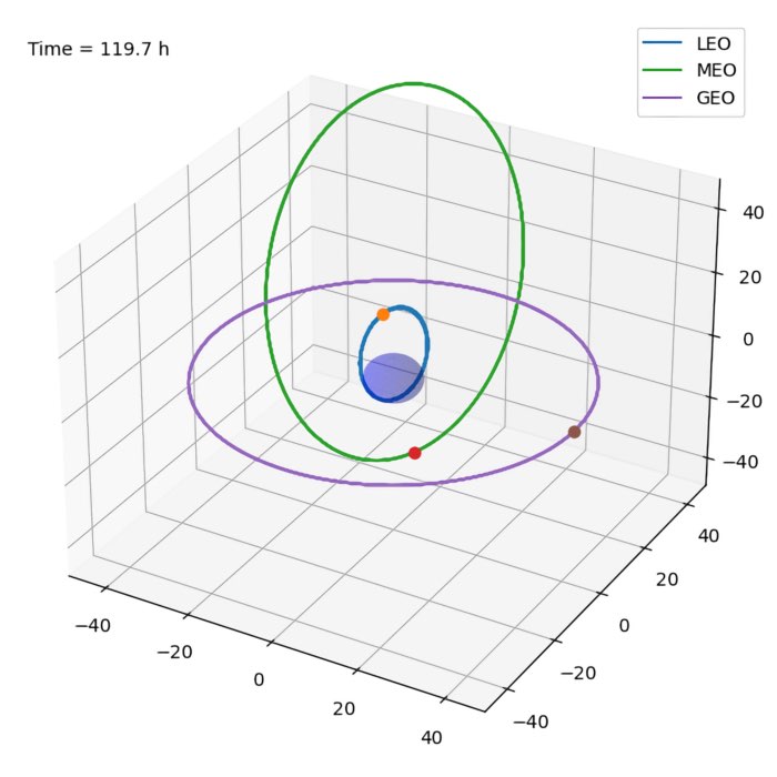
The Python code below implements the RK4 method as described above. It simulates the motion of three artificial satellites around the Earth. The satellites are located in low Earth orbit (LEO), medium Earth orbit (MEO), and geostationary Earth orbit (GEO). The initial conditions for each satellite are defined in the params list and you can extend it with further satellite if you’d like to. The satellites start at the perigee of an elliptical orbit with semi-major axis a and eccentricity e. The velocity at perigee is calculated to ensure the orbit is elliptical. The orbit is inclined at an angle i from the x-y-plane. m corresponds to the masses of each simulated satellite, and M_Earth corresponds to the mass of the Earth with M_Earth $\gg$ m.
For reproducibility:
conda create -n orbit -y python=3.7
conda activate orbit
conda install mamba -y
mamba install -y numpy matplotlib scikit-learn ipykernel
Here is the code:
import numpy as np
import matplotlib.pyplot as plt
from mpl_toolkits.mplot3d import Axes3D
import matplotlib.animation as animation

# Constants:
G = 6.67430e-11  # gravitational constant in m^3 kg^-1 s^-2
M_earth = 5.972e24  # Earth's mass in kg
R_earth = 6.371e6  # Earth's radius in m
dt = 200  # time step in seconds

# List of (a, e, i, m, label) parameters for each satellite:
params = [
    (7.0e6, 0.0, 51.6, 420.0, 'LEO'),
    (26.56e6, 0.01, 55, 2000.0, 'MEO'),
    (42.164e6, 0.0, 0, 2000.0, 'GEO')
    # add more satellites if you like to
]

# Function to calculate initial conditions:
def calculate_initial_conditions(a, e, i, m):
    v_perigee = np.sqrt(G * (M_earth + m) * (1 + e) / (a * (1 - e)))  # Velocity at perigee
    return [a * (1 - e), 0, a * np.sin(np.radians(i)), 0, v_perigee * np.cos(np.radians(i)), v_perigee * np.sin(np.radians(i))]

def create_satellites(params):
    satellites = []
    for idx, (a, e, i, m, label) in enumerate(params):
        satellites.append({
            'name': f'sat{idx+1}',
            'a': a,
            'e': e,
            'i': i,
            'm': m,
            'label': label,
            'state0': calculate_initial_conditions(a, e, i, m)
        })
    return satellites

# "Generate" the satellites:
satellites = create_satellites(params)

# Time setup:
t_max = 10 * np.pi * np.sqrt(max(sat['a'] for sat in satellites)**3 / (G * M_earth))  # Period of the furthest satellite
t = np.arange(0, t_max, dt)

# RK4 step:
def rk4_step(func, state, t, dt, m):
    k1 = func(state, t, m)
    k2 = func(state + dt/2 * k1, t + dt/2, m)
    k3 = func(state + dt/2 * k2, t + dt/2, m)
    k4 = func(state + dt * k3, t + dt, m)
    return state + dt / 6 * (k1 + 2*k2 + 2*k3 + k4)

# System of differential equations:
def func(state, t, m):
    x, y, z, vx, vy, vz = state
    r = np.sqrt(x**2 + y**2 + z**2)
    ax = - G * (M_earth + m) * x / r**3
    ay = - G * (M_earth + m) * y / r**3
    az = - G * (M_earth + m) * z / r**3
    return np.array([vx, vy, vz, ax, ay, az])

# Solve system of equations:
for sat in satellites:
    path = [sat['state0']]
    for t_i in t[1:]:
        path.append(rk4_step(func, path[-1], t_i, dt, sat['m']))
    sat['path'] = np.array(path)

# Convert units to thousand km:
for sat in satellites:
    sat['path'][:,:3] /= 1e6
    sat['a'] /= 1e6
R_earth /= 1e6

# Calculate the maximum extent of any satellite's path:
max_extent = max(np.max(np.sqrt(np.sum(sat['path'][:,:3]**2, axis=1))) for sat in satellites)/2

# Animation:
fig = plt.figure(figsize=(6,6))
ax = fig.add_subplot(111, projection='3d')

# Draw Earth:
u = np.linspace(0, 2 * np.pi, 100)
v = np.linspace(0, np.pi, 100)
x = R_earth * np.outer(np.cos(u), np.sin(v))
y = R_earth * np.outer(np.sin(u), np.sin(v))
z = R_earth * np.outer(np.ones(np.size(u)), np.cos(v))
ax.plot_surface(x, y, z, color='b', alpha=0.25)

# Create lines and points for each satellite:
lines = []
points = []
for sat in satellites:
    sat_line, = ax.plot([], [], [], label=sat['label'])
    lines.append(sat_line)
    sat_point, = ax.plot([], [], [], 'o')
    points.append(sat_point)
time_text = ax.text2D(0.02, 0.95, '', transform=ax.transAxes)
ax.legend()

def init():
    ax.set_xlim(-1.2*max_extent, 1.2*max_extent)
    ax.set_ylim(-1.2*max_extent, 1.2*max_extent)
    ax.set_zlim(-1.2*max_extent, 1.2*max_extent)
    plt.tight_layout()
    for line, point in zip(lines, points):
        line.set_data([], [])
        line.set_3d_properties([])
        point.set_data([], [])
        point.set_3d_properties([])
    time_text.set_text('')
    return lines + points + [time_text]

def update(frame):
    for sat, line, point in zip(satellites, lines, points):
        line.set_data(sat['path'][:frame,0], sat['path'][:frame,1])
        line.set_3d_properties(sat['path'][:frame,2])
        point.set_data(sat['path'][frame,0], sat['path'][frame,1])
        point.set_3d_properties(sat['path'][frame,2])
    time_text.set_text(f'Time = {frame*dt/3600:.1f} h')
    plt.tight_layout()
    return lines + points + [time_text]

ani = animation.FuncAnimation(fig, update, frames=len(t), init_func=init, blit=True, interval=1)
ani.save('satellites_orbit.gif', writer='imagemagick', fps=10)
plt.show()
This is the simulation result:
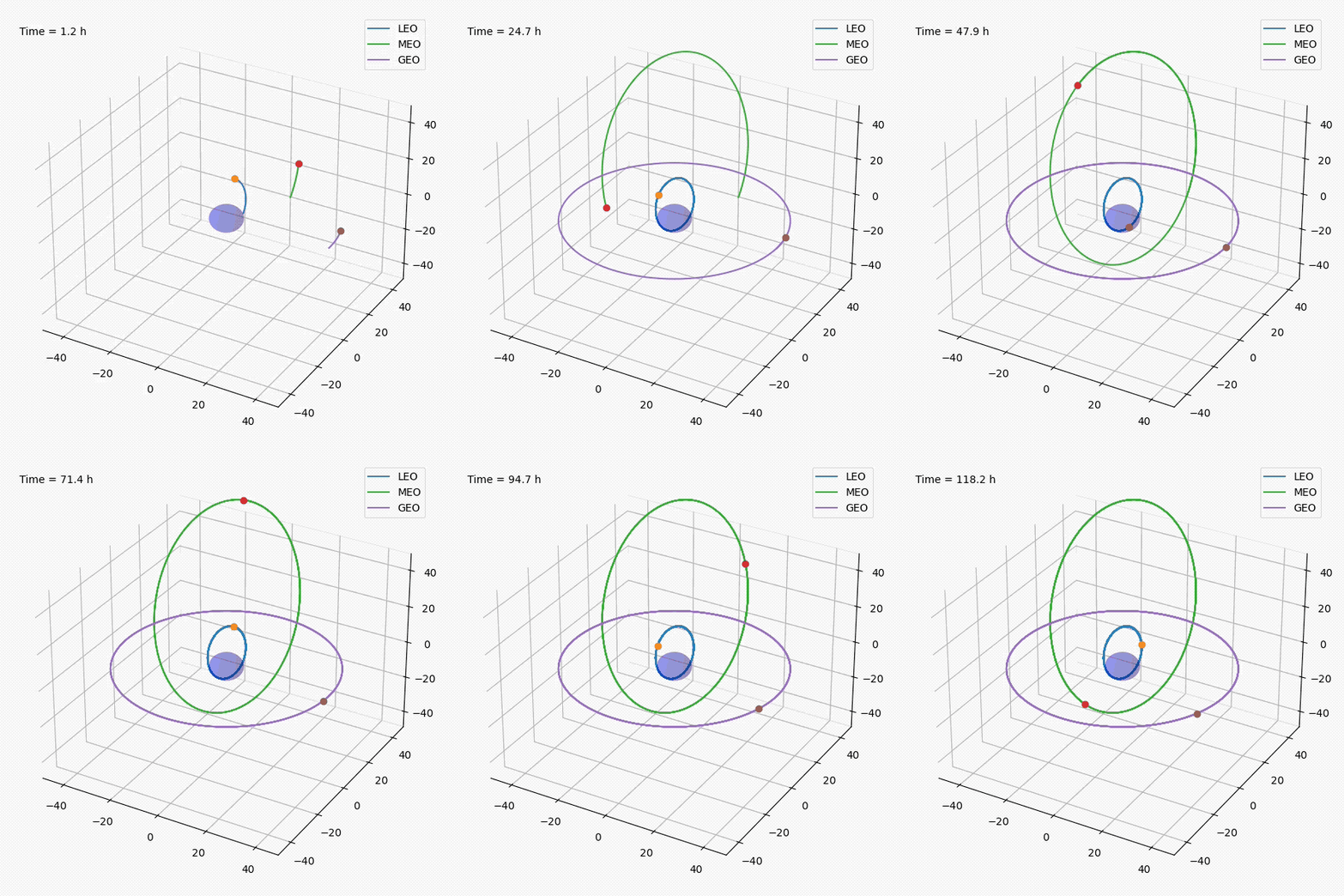 Simulated orbits of three satellites around the Earth. The satellites are located in low Earth orbit (LEO), medium Earth orbit (MEO), and geostationary Earth orbit (GEO). The orbits are inclined at different angles from the x-y-plane. The animation shows the orbits of the satellites over a period of 10 times the period of the furthest satellite. The Earth is shown in blue.
Conclusion
Understanding the dynamics of celestial bodies is a fascinating area of study, involving problems such as the $n$-body problem. While the $n$-body problem presents significant challenges in terms of analytical solutions, numerical methods like the RK4 method allow us to approximate the motion of multiple bodies. The provided Python code for simulating the orbits of satellites around the Earth demonstrates, in a simplified manner, how the RK4 method can be used to solve the two-body problem. Bear in mind, that it does not account for all real-world factors that may affect satellite orbits. Feel free to expand it upon for more accurate and comprehensive simulations.
The entire code used in this post is available in this GitHub repositoryꜛ.
If you have any questions or suggestions, feel free to leave a comment below.
Comments
Commenting on this post is currently disabled.
Comments on this website are based on a Mastodon-powered comment system. Learn more about it here.