Runge-Kutta methods for solving ODEs
In physics and computational mathematics, numerical methods for solving ordinary differential equations (ODEs) are of central importance. Among these, the family of Runge-Kutta methods stands out due to its versatility and robustness. In this post we compare the first four orders of the Runge-Kutta methods, namely RK1 (Euler’s method), RK2, RK3, and RK4.
Mathematical background
Runge-Kutta methods are a family of numerical methods for solving first-order ordinary differential equations (ODEs). They are based on the Taylor series expansion of the solution $y(t)$ around the current point $t_n$. The basic concept of Runge-Kutta methods revolves around the iterative evaluation of the derivative at several points to achieve a more accurate estimation of the function value. As the order of the method increases, so does the number of evaluations per step and therefore the overall accuracy, but at the expense of computational cost.
RK1: Euler’s Method
Euler’s method, known as the first order Runge-Kutta method (RK1), is the simplest in this family. It works by using the derivative at the current point to estimate the next point:
\[\begin{align*} k_1 &= h \cdot f(t_n, y_n) \\ y_{n+1} &= y_n + k_1 \end{align*}\]$y_{n+1}$ is the next value, $y_n$ is the current value, $f(t_n, y_n)$ is the derivative at the current point, and $h$ is the step size.
RK2
The second order Runge-Kutta method (RK2) incorporates the derivative at the midpoint of the interval to achieve better accuracy:
\[\begin{align*} k_1 &= h \cdot f(t_n, y_n) \\ k_2 &= h \cdot f\left(t_n + \frac{h}{2}, y_n + \frac{k_1}{2}\right) \\ y_{n+1} &= y_n + k_2 \end{align*}\]RK3
The third order Runge-Kutta method (RK3) adds another midpoint derivative evaluation:
\[\begin{align*} k_1 &= h \cdot f(t_n, y_n) \\ k_2 &= h \cdot f\left(t_n + \frac{h}{2}, y_n + \frac{k_1}{2}\right) \\ k_3 &= h \cdot f(t_n + h, y_n - k_1 + 2k_2) \\ y_{n+1} &= y_n + \frac{k1 + 4k_2 + k_3}{6} \end{align*}\]RK4
Finally, the fourth order Runge-Kutta method (RK4) includes yet another derivative estimation, and offers a more balanced combination of the four derivative evaluations:
\[\begin{align*} k_1 &= h \cdot f(t_n, y_n) \\ k_2 &= h \cdot f\left(t_n + \frac{h}{2}, y_n + \frac{k_1}{2}\right) \\ k_3 &= h \cdot f\left(t_n + \frac{h}{2}, y_n + \frac{k_2}{2}\right) \\ k_4 &= h \cdot f(t_n + h, y_n + k3) \\ y_{n+1} &= y_n + \frac{k_1 + 2k_2 + 2k_3 + k_4}{6} \end{align*}\]Higher order ODEs
Standard Runge-Kutta methods are typically designed to solve systems of first-order ODEs. However, higher-order ODEs can be transformed into an equivalent system of first-order ODEs, allowing us to apply Runge-Kutta methods to solve them.
To convert a higher-order ODE into a system of first-order ODEs, we usually introduce additional variables to represent the derivatives of the original unknown function. For example, consider a second-order ODE:
\[y''(t) = f(t, y(t), y'(t))\]To convert this into a system of first-order ODEs, we introduce a new variable $v(t)$ to represent the derivative of $y(t)$:
\[y'(t) = v(t)\]Now, we have two first-order ODEs:
\[y'(t) = v(t)\] \[v'(t) = f(t, y(t), v(t))\]We can apply Runge-Kutta methods to solve this system of first-order ODEs numerically. By integrating the equations simultaneously, we obtain a numerical approximation for both $y(t)$ and $v(t)$, which represent the solution to the original second-order ODE.
Therefore, although Runge-Kutta methods are designed for first-order ODEs, we can transform higher-order ODEs into an equivalent system of first-order ODEs to utilize these methods effectively.
Example: Solving a simple ODE
Below is the Python implementation of each method applied to the differential equation $y’ = y$ with the exact solution $y(t) = e^t$. To assess the accuracy of the numerical solution, we calculate the mean squared error (MSE) between the exact solution and the numerical solution.
For reproducibility:
conda create -n rungekutta -y python=3.7
conda activate rungekutta
conda install -y numpy matplotlib scikit-learn ipykernel
Here is the code:
# Define the function
def f(t, y):
    return y

# Exact solution
def y_exact(t):
    return np.exp(t)

# Define the Runge-Kutta methods
def rk1(y, t, dt, derivs):
    k1 = dt * derivs(t, y)
    y_next = y + k1
    return y_next

def rk2(y, t, dt, derivs):
    k1 = dt * derivs(t, y)
    k2 = dt * derivs(t + dt / 2, y + k1 / 2)
    y_next = y + k2
    return y_next

def rk3(y, t, dt, derivs):
    k1 = dt * derivs(t, y)
    k2 = dt * derivs(t + dt / 2, y + k1 / 2)
    k3 = dt * derivs(t + dt, y - k1 + 2 * k2)
    y_next = y + (k1 + 4 * k2 + k3) / 6
    return y_next

def rk4(y, t, dt, derivs):
    k1 = dt * derivs(t, y)
    k2 = dt * derivs(t + dt / 2, y + k1 / 2)
    k3 = dt * derivs(t + dt / 2, y + k2 / 2)
    k4 = dt * derivs(t + dt, y + k3)
    y_next = y + (k1 + 2 * k2 + 2 * k3 + k4) / 6
    return y_next

# Define parameters
t_start = 0.0
t_end = 2.0
N = 10  # number of steps
h = (t_end - t_start) / N  # step size
t_values = np.linspace(t_start, t_end, N+1)

# Initial condition
y_0 = 1.0

# Solve the ODE using different methods and calculate MSE
y_values_rk = dict()
mse_values = dict()

for method, name in [(rk1, 'RK1'), (rk2, 'RK2'), (rk3, 'RK3'), (rk4, 'RK4')]:
    y_values = np.zeros(N+1)
    y_values[0] = y_0
    for i in range(N):
        y_values[i+1] = method(y_values[i], t_values[i], h, f)
    y_values_rk[name] = y_values
    mse_values[name] = mean_squared_error(y_exact(t_values), y_values)

# Plot the results
plt.figure(figsize=(6, 5))
plt.plot(t_values, y_exact(t_values), label='Exact solution', linestyle='--', color='k', lw=4)
for name in ['RK1', 'RK2', 'RK3', 'RK4']:
    plt.plot(t_values, y_values_rk[name], label=f'{name} (MSE: {mse_values[name]:.2e})')
plt.xlabel('t')
plt.ylabel('y')
plt.title(f"Solving $y' = y$ with step-size h={h}")
plt.legend()
plt.grid(True)
plt.tight_layout()
plt.savefig(f'runge_kutta_method_exponential_h_{np.round(h, 2)}.png', dpi=200)
plt.show()
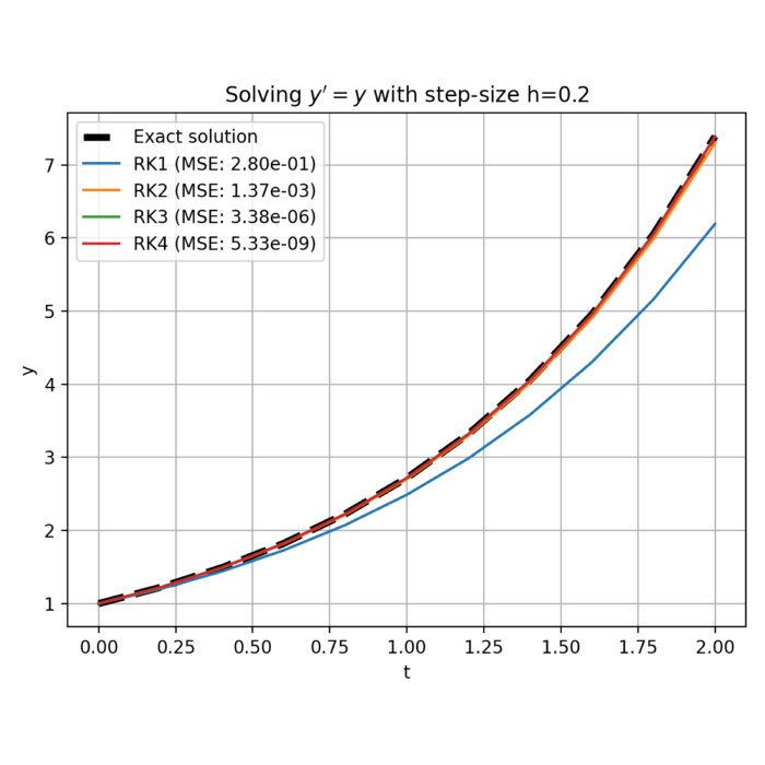
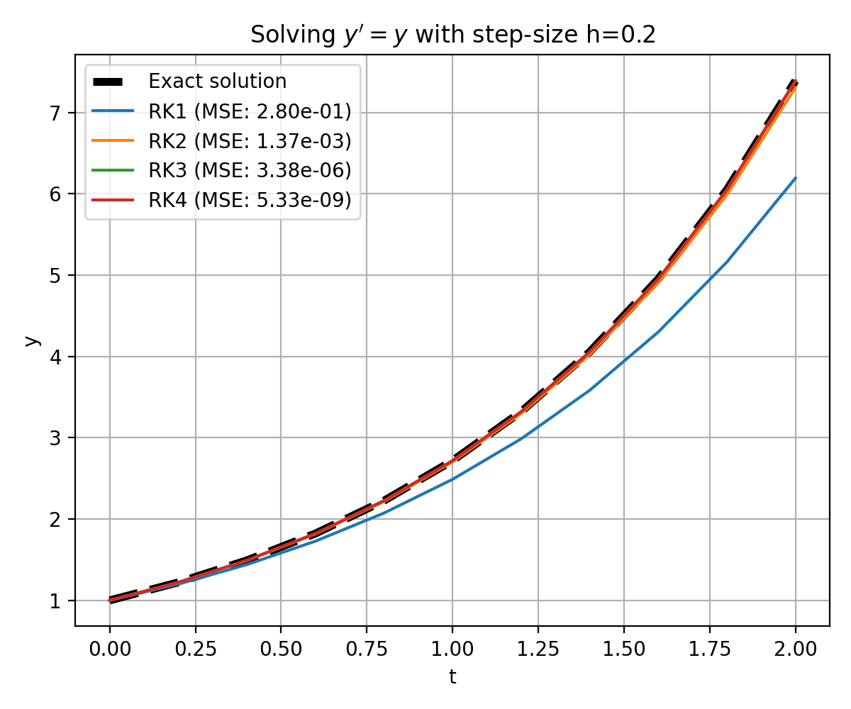 The solution to the ODE $y’ = y$ with initial condition $y(0) = 1$ is $y(t) = e^t$. The plot shows the exact solution (dashed line) and the numerical solutions using the Runge-Kutta methods RK1 to RK4 with step-size $h=0.2$. The mean squared error (MSE) for each method is shown in the legend. The MSE decreases with increasing order of the method, indicating that the higher order methods provide more accurate solutions. However, the computational cost also increases with the order of the method. Hence, the choice of method should balance accuracy requirements and computational efficiency.
The plot shows the exact solution (dashed line) and the numerical solutions using the Runge-Kutta methods RK1 to RK4 with step-size $h=0.2$. The mean squared error (MSE) for each method is shown in the legend. The MSE decreases with increasing order of the method, indicating that the higher order methods provide more accurate solutions. However, the computational cost also increases with the order of the method, especially for more complex problems and longer simulation times.
Another factor that controls the accuracy of the numerical solution is the step size $h$. The smaller the step size, the more accurate the solution. However, the computational cost increases with decreasing step size. The following plot shows the same simulation, but with a smaller step size $h=0.02$. Note, how the Euler method (RK1) now provides a more accurate solution (but still not matching the exact solution and the higher-order RK methods):
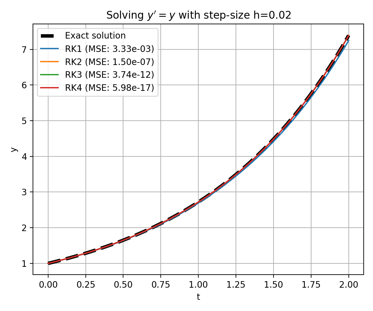 Similar to the previous plot, but with step-size $h=0.02$.
Example: Simple pendulum
For the pendulum with small angle approximation, the ODE is $y’’ = - \sin(y) \approx -y$. The motion is simple harmonic and the solution to the ODE is a sine or cosine function. Assuming zero initial velocity and initial angle $y_0$, the exact solution would be $y(t) = y_0 \cos(t)$.
Since the underlying ODE is second-order, we first need to rewrite it as a system of two first-order ODEs, which allows us to apply the Runge-Kutta methods. As a first step, we rewrite the ODE as:
\[\frac{d^2y}{dt^2} + y = 0\]We now introduce an auxiliary variable $v$ such that $v = \frac{dy}{dt}$. This leads to two first-order ODEs:
\[\frac{dy}{dt} = v\] \[\frac{dv}{dt} = -y\]With this system of first-order ODEs, we can now apply the Runge-Kutta methods to solve the pendulum problem.
def pendulum(t, state):
    y, v = state
    dydt = v
    dvdt = -y
    return np.array([dydt, dvdt])

# Exact solution
def y_exact(t):
    return state_0[0] * np.cos(t)

# Define parameters
t_start = 0.0
t_end = 10.0
N = 20  # number of steps
h = (t_end - t_start) / N  # step size
t_values = np.linspace(t_start, t_end, N+1)

# Initial condition
state_0 = np.array([0.1, 0])  # small initial angle, zero initial velocity

# Solve the ODE using different methods and calculate MSE
state_values_rk = dict()
mse_values = dict()

for method, name in [(rk1, 'RK1'), (rk2, 'RK2'), (rk3, 'RK3'), (rk4, 'RK4')]:
    state_values = np.zeros((N+1, 2))
    state_values[0] = state_0
    for i in range(N):
        state_values[i+1] = method(state_values[i], t_values[i], h, pendulum)
    state_values_rk[name] = state_values
    # Calculate MSE for the angle
    mse_values[name] = mean_squared_error(np.sin(t_values), state_values[:, 0])

# Calculate MSE and plot the results
plt.figure(figsize=(6, 5))
plt.plot(t_values, y_exact(t_values), label='Exact solution', linestyle='--', color='k', lw=4)
for name in ['RK1', 'RK2', 'RK3', 'RK4']:
    mse_values[name] = mean_squared_error(y_exact(t_values), state_values_rk[name][:, 0])
    plt.plot(t_values, state_values_rk[name][:, 0], label=f'{name} (MSE: {mse_values[name]:.2e})')
plt.xlabel('t')
plt.ylabel('y (angle)')
plt.title(f"Solving $y'' = - \sin(y) \approx -y$ (pendulum) with step-size h={h}")
plt.legend()
plt.grid(True)
plt.tight_layout()
plt.savefig(f'runge_kutta_method_pendulum_h_{np.round(h, 2)}.png', dpi=200)
plt.show()
The definitions of RK1 to RK4 remain unchanged, which is why they are not repeated in the code above. However, the derivative function needed to be modified to handle a system of differential equations with two variables, $y$ and $v$, corresponding to the angle and angular velocity of the pendulum, respectively. The function pendulum takes the current time t and state vector state (an array with $y$ and $v$) as inputs and returns the derivatives $\frac{dy}{dt} = v$ and $\frac{dv}{dt} = -y$. The initial conditions for the pendulum problem now have to include both the initial angle $y_0$ and initial angular velocity $v_0$ as elements of the state_0 array. In the Runge-Kutta methods, when calculating the intermediate values $k_1$, $k_2$, $k_3$, and $k_4$, we need to call the pendulum function with the current time t and current state state. The function will then return the derivatives $\frac{dy}{dt}$ and $\frac{dv}{dt}$, which are used to update the state accordingly. When updating the state in the Runge-Kutta methods, we need to update both $y$ and $v$ using the respective derivatives calculated in the pendulum function.
From the plots below, we again see that the higher order methods provide more accurate solutions. The Euler method (RK1) is the least accurate, but also the most computationally efficient. The RK4 method is the most accurate, but also the most computationally expensive. The RK2 and RK3 methods provide a good balance between accuracy and computational cost. Note, how the solution, especially for the Euler method (RK1), improves with decreasing step size $h$.
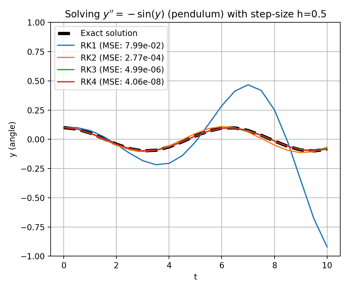 The solution to the ODE $y’’ = -y$ (simple pendulum with small angle approximation) with initial condition $y(0) = 0.1$ and $y’(0) = 0$ is $y(t) = y_0 \cos(t)$. The plot shows the exact solution (dashed line) and the numerical solutions using the Runge-Kutta methods RK1 to RK4 with step-size $h=0.5$.
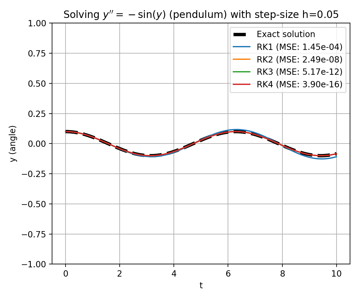 Same as previous plot, but with step-size $h=0.05$.
Built-in numerical integrator in Python
There are several libraries available in Python that include numerical integrators, such as the Runge-Kutta methods, making it easier to solve differential equations. One popular library is SciPy, which provides a sub-module called scipy.integrate for numerical integration. Here’s an example of how you can use the solve_ivp function from scipy.integrate to solve the simple pendulum problem:
import numpy as np
from scipy.integrate import solve_ivp
import matplotlib.pyplot as plt

def pendulum(t, state):
    y, v = state
    return [v, -y]  # Return the derivatives [dy/dt, dv/dt]

# Define the initial conditions and time span
t0 = 0.0
t_end = 10.0
y0 = 0.1  # Initial angle
v0 = 0.0  # Initial angular velocity

# Define the step size
step_size = 0.01

# Solve the differential equation using solve_ivp
sol = solve_ivp(pendulum, [t0, t_end], [y0, v0], max_step=step_size)

# Extract the solution
t_values = sol.t
y_values = sol.y[0]  # Angle values

# Calculate the exact solution
exact_solution = y0 * np.cos(t_values)

plt.figure(figsize=(6, 5))
plt.plot(t_values, exact_solution, label='Exact solution', c='k', lw=4)
plt.plot(t_values, y_values, label='Numerical solution (RK4/5)', c='cyan', ls='--', lw=2)
plt.xlabel('t')
plt.ylabel('y (angle)')
plt.title('Simple pendulum solution solved with solve_ivp')
plt.legend()
plt.grid(True)
plt.tight_layout()
plt.savefig('pendulum_solve_ivp.png', dpi=200)
plt.show()
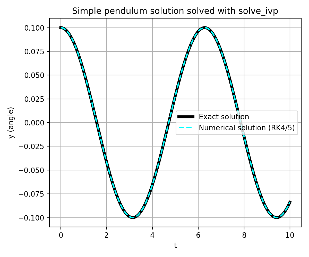 Solution of the simple pendulum using the
 solve_ivp function from scipy.integrate. The exact solution (dashed line) and the numerical solution (dotted line) are shown.
solve_ivp uses the Dormand-Prince method as the default numerical integration algorithm. The Dormand-Prince method, also known as the Runge-Kutta 4/5 method, is a popular adaptive-step-size Runge-Kutta method that provides accurate and efficient solutions for a wide range of differential equations.
Conclusion
In conclusion, the Runge-Kutta (RK) methods are effective numerical integration techniques used to solve first-order ordinary differential equations (ODEs). The accuracy of RK methods depends on the order of the method and the step size. Higher-order RK methods and smaller step sizes offer greater accuracy, but require more computational effort. Thus, the choice of method should and step-size balance accuracy requirements and computational efficiency. Smaller step sizes improve accuracy at the cost of increased computational time. Python’s built-in integrators, like solve_ivp, provide convenient options for numerical integration. By selecting an appropriate RK method and adjusting the step size, accurate and efficient solutions can be obtained for a wide range of ODE problems.
The entire code used in this post is available in this GitHub repositoryꜛ.
If you have any questions or suggestions, feel free to leave a comment below.
If you want to see more RK examples, check out my next post on the Lorenz system and the Runge-Kutta methods.




comments