Rössler attractor

Unlike the Lorenz attractor which emerges from the dynamics of convection rolls, the Rössler attractor, introduced by Otto Rössler in 1976, does not describe a physical system found in nature. Instead, it is a mathematical construction designed to illustrate and study the behavior of chaotic systems in a simpler, more accessible manner. In this post, we explore how we can quickly simulate this strange attractor using simple Python code.

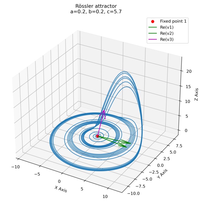
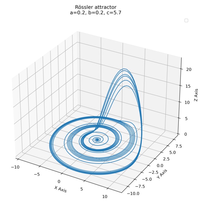The Rössler attractor with parameters $a = 0.2$, $b = 0.2$, and $c = 5.7$.

Mathematical foundation and dynamics

The Rössler attractor is defined by a set of three non-linear ordinary differential equations (ODEs):

\[\begin{align*} \dot{x} &= -y - z \\ \dot{y} &= x + ay \\ \dot{z} &= b + z(x - c) \end{align*}\]

where $x$, $y$, and $z$ represent the system state variables, and $a$, $b$, and $c$ are parameters that dictate the system’s behavior. Typically, the parameters are chosen such that the system exhibits chaotic behavior; a common choice is $a = 0.2$, $b = 0.2$, and $c = 5.7$. $x$, $y$, and $z$ are state variables, representing a point in the phase space, evolving over time according to the differential equations provided.

The dynamics of the Rössler attractor are characterized by an interplay between two key motions: A rotation around an unstable equilibrium point and an expansion away from this point followed by a sudden collapse back towards it. This behavior results in the attractor’s distinctive spiral shape in the $x-y$ plane, combined with an oscillation in the $z$ dimension.

Python implementation

Simulating the Rössler attractor requires solving the system of ODEs using a numerical integration method. Here, we use the Runge-Kutta 4th order method (RK4) to solve the ODEs. RK4 is a widely used technique for the numerical solution of systems of ODEs, renowned for its balance between computational efficiency and accuracy.

The RK4 method approximates the solution of the system at time $t + \Delta t$ from a known state at time $t$ by calculating four incremental changes ($k_1$, $k_2$, $k_3$, $k_4$) based on the evaluation of the ODEs at various points within the interval $\Delta t$. These incremental changes are defined as:

\[\begin{align*} k_1 &= f(t, \mathbf{y}), \\ k_2 &= f\left(t + \frac{\Delta t}{2}, \mathbf{y} + \frac{\Delta t}{2} k_1\right), \\ k_3 &= f\left(t + \frac{\Delta t}{2}, \mathbf{y} + \frac{\Delta t}{2} k_2\right), \\ k_4 &= f(t + \Delta t, \mathbf{y} + \Delta t k_3), \end{align*}\]

where $f(t, \mathbf{y})$ represents the right-hand side of the ODEs, and $\mathbf{y}$ is the vector of state variables $(x, y, z)$ at time $t$.

The new approximation $\mathbf{y}(t + \Delta t)$ is then calculated by the weighted sum of these increments:

\[\mathbf{y}(t + \Delta t) = \mathbf{y}(t) + \frac{\Delta t}{6}(k_1 + 2k_2 + 2k_3 + k_4).\]

This method incrementally integrates the system forward in time, using the local rates of change of the system to create an accurate trajectory of the state vector in phase space.

Translating these mathematical concepts into Python code, we can define a function roessler_attractor to represent the Rössler attractor’s dynamics and another function rk4_step to apply the RK4 method to advance the system’s state by a time step $dt$:

# function to calculate the derivatives:
def roessler_attractor(state, a, b, c):
    x, y, z = state
    dx = -y - z
    dy = x + a*y
    dz = b + z*(x - c)
    return np.array([dx, dy, dz])

# RK4 step function:
def rk4_step(state, dt, a, b, c):
    k1 = roessler_attractor(state, a, b, c)
    k2 = roessler_attractor(state + dt/2 * k1, a, b, c)
    k3 = roessler_attractor(state + dt/2 * k2, a, b, c)
    k4 = roessler_attractor(state + dt * k3, a, b, c)
    return state + dt / 6 * (k1 + 2*k2 + 2*k3 + k4)

The roessler_attractor function takes the current state of the system (comprised of $x$, $y$, and $z$) and the parameters $a$, $b$, and $c$ that define the attractor’s behavior. The function calculates the derivatives $\dot{x}$, $\dot{y}$, and $\dot{z}$, which represent the rate of change in the system’s state, effectively describing its trajectory through phase space.

The rk4_step function applies the RK4 method to advance the system’s state by a time step $dt$. This method calculates the four estimates ($k1$, $k2$, $k3$, and $k4$) of the system’s state at different points within the time step and combines them to produce a weighted average that approximates the system’s state at the end of the time step.

To calculate the trajectory of the Rössler attractor, we simply run a loop that iterates over time, applying the rk4_step function at each time step:

# generating the trajectory:
path = np.zeros((step_count, 3))
path[0] = [x0, y0, z0]
for i in range(1, step_count):
    path[i] = rk4_step(path[i-1], dt, a, b, c)

where step_count is the number of time steps, and dt is the time step size. The initial state of the system is defined by the variables x0, y0, and z0.

The full Python code to simulate the Rössler attractor including plot commands and the part to generate a GIF animation is as follows:

# %% IMPORTS
import numpy as np
import matplotlib.pyplot as plt
from mpl_toolkits.mplot3d import Axes3D
import matplotlib.animation as animation

# %% PARAMETERS
# parameters for the Rössler attractor:
a, b, c = 0.2, 0.2, 5.7

# time step and total number of steps (affects the duration of the calculation and the gif):
dt = 0.03
step_count = 5000

# initial condition:
x0, y0, z0 = 0.0, 0.0, 0.0

# %% FUNCTIONS
# function to calculate the derivatives:
def roessler_attractor(state, a, b, c):
    x, y, z = state
    dx = -y - z
    dy = x + a*y
    dz = b + z*(x - c)
    return np.array([dx, dy, dz])

# RK4 step function:
def rk4_step(state, dt, a, b, c):
    k1 = roessler_attractor(state, a, b, c)
    k2 = roessler_attractor(state + dt/2 * k1, a, b, c)
    k3 = roessler_attractor(state + dt/2 * k2, a, b, c)
    k4 = roessler_attractor(state + dt * k3, a, b, c)
    return state + dt / 6 * (k1 + 2*k2 + 2*k3 + k4)

# %% MAIN
# generating the trajectory:
path = np.zeros((step_count, 3))
path[0] = [x0, y0, z0]
for i in range(1, step_count):
    path[i] = rk4_step(path[i-1], dt, a, b, c)

# %% PLOTTING THE ATTRACTOR'S FINAL STATE
fig = plt.figure(figsize=(10, 7))
ax = fig.add_subplot(111, projection='3d')
ax.plot(path[:, 0], path[:, 1], path[:, 2], lw=0.5)
ax.set_xlabel("X Axis")
ax.set_ylabel("Y Axis")
ax.set_zlabel("Z Axis")
ax.set_title(f"Rössler attractor\na={a}, b={b}, c={c}")
plt.tight_layout()
plt.savefig("roessler_attractor.png", dpi=300)
plt.show()

# %% PLOTTING THE ANIMATION
fig = plt.figure()
ax = fig.add_subplot(111, projection='3d')

# adding a text object for time display:
time_text = ax.text2D(0.05, 0.95, '', transform=ax.transAxes)

def init():
    ax.set_xlim((np.min(path[:,0]), np.max(path[:,0])))
    ax.set_ylim((np.min(path[:,1]), np.max(path[:,1])))
    ax.set_zlim((np.min(path[:,2]), np.max(path[:,2])))
    time_text.set_text('')
    return fig,

def update(num, path, line, time_text):
    line.set_data(path[:num, 0], path[:num, 1])
    line.set_3d_properties(path[:num, 2])
    # Update time display with current simulation time
    time_text.set_text(f'Time = {num*dt:.2f} s')
    print(f"Current step: {num}, Time: {num*dt:.2f} s")
    return line, time_text

line, = ax.plot([], [], [], lw=1)
ani = animation.FuncAnimation(fig, update, step_count, fargs=(path, line, time_text),
                              init_func=init, blit=False, interval=1)

# run and save the animation: 
ani.save('roessler_attractor_with_time.gif', writer='imagemagick', fps=30)
plt.show()

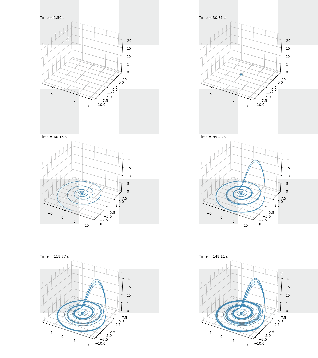The Rössler attractor simulated with parameters $a = 0.2$, $b = 0.2$, and $c = 5.7$. The attractor evolves slowly during the first $\sim$20 seconds, but then the dynamics become faster.

Conclusion

The Rössler attractor is a fascinating example of a chaotic dynamical system that exhibits complex, unpredictable behavior. By simulating the attractor using simple Python code, we can gain insight into the dynamics of chaotic systems and explore the interplay between the system’s state variables. The Rössler attractor is a valuable tool for studying the behavior of chaotic systems, as well as biological systems, chemical reactions, and engineering systems, and provides a simple yet powerful example of the rich dynamics that can emerge from non-linear systems.

You can find the complete code for this post also in this GitHub repositoryꜛ.

Info: In this post, I analyze the Rössler attractor by calculating its nullclines and fixed points. By investigating the local dynamics around the fixed points using eigenvalues and eigenvectors, we gain even further insights into the attractor’s behavior.