Solving the Lorenz system using Runge-Kutta methods

In my previous post, I introduced the Runge-Kutta methods for numerically solving ordinary differential equations (ODEs), that are challenging to solve analytically. In this post, we apply the Runge-Kutta methods to solve the Lorenz system. The Lorenz system is a set of differential equations known for its chaotic behavior and non-linear dynamics. By utilizing the Runge-Kutta methods, we can effectively simulate and analyze the intricate dynamics of this system.

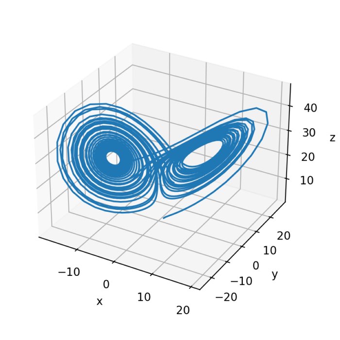
The Lorenz System

The Lorenz system was introduced by Edward Lorenz in 1963 as a simplified model for atmospheric convection. It consists of three coupled non-linear differential equations that describe the evolution of variables representing the state of the system. The Lorenz system is widely studied due to its intriguing chaotic behavior and its ability to exhibit sensitive dependence on initial conditions.

Furthermore, the Lorenz system is also a representation of a fascinating phenomenon known as the “butterfly effect.” Perhaps you already learned about the effect from the movie “The Butterfly Effect” from 2004, starring Ashton Kutcher. The movie explores the idea that even minute changes in the past can have a profound impact on the future. The butterfly effect is a metaphor for the sensitive dependence on initial conditions, which is a defining characteristic of chaotic systems. In general, it refers to the idea that small changes in the initial conditions of a system can lead to dramatically different outcomes over time. It draws its name from the poetic notion that the flap of a butterfly’s wings in Brazil could potentially set off a chain of events that eventually culminate in a tornado in Texas.

By studying and simulating the Lorenz system, we can gain insights into the chaotic behavior and intricate dynamics that underlie complex systems. The application of Runge-Kutta methods enables us to approximate the solutions of the Lorenz system and explore its behavior.

Mathematical representation

The Lorenz system can be mathematically described via the following set of first-order differential equations:

\[\begin{align*} \frac{dx}{dt} &= \sigma (y - x) \\ \frac{dy}{dt} &= x(\rho - z) - y \\ \frac{dz}{dt} &= xy - \beta z \\ \end{align*}\]

Here, $x$, $y$, and $z$ represent the state variables, $t$ is time, and $\sigma$, $\rho$, and $\beta$ are the system parameters. These parameters control the dynamics of the system and influence its behavior. Values such as $\sigma = 10$, $\rho = 28$, and $\beta = 8/3$ are commonly used to simulate the Lorenz system. Also the setting of the initial conditions is of importance and determines the behavior of the system. For example, the initial conditions $x(0) = 1$, $y(0) = 1$, and $z(0) = 1$ lead to chaotic behavior, whereas the initial conditions $x(0) = 0$, $y(0) = 0$, and $z(0) = 0$ lead to a stable equilibrium.

Solving the Lorenz system analytically is challenging due to its non-linear nature. Numerical methods are therefore employed to approximate its solutions. Runge-Kutta methods, a class of numerical integrators, are particularly useful for solving systems of ordinary differential equations like the Lorenz system. These methods allow us to step forward in time and estimate the state variables at each time step based on the current state and the derivative information. If you want to learn more about Runge-Kutta methods, check my previous post.

Runge-Kutta equations for the Lorenz System

The Runge-Kutta methods provide a systematic approach to approximate the solution of ordinary differential equations. The according equations for the Lorenz system are given by:

For RK1:

\[\begin{align*} k_1 &= h \cdot f(t_n, \mathbf{y}_n) \\ \mathbf{y}_{n+1} &= \mathbf{y}_n + k_1 \end{align*}\]

For RK2:

\[\begin{align*} k_1 &= h \cdot f(t_n, \mathbf{y}_n) \\ k_2 &= h \cdot f\left(t_n + \frac{h}{2}, \mathbf{y}_n + \frac{k_1}{2}\right) \\ \mathbf{y}_{n+1} &= \mathbf{y}_n + k_2 \end{align*}\]

For RK3:

\[\begin{align*} k_1 &= h \cdot f(t_n, \mathbf{y}_n) \\ k_2 &= h \cdot f\left(t_n + \frac{h}{2}, \mathbf{y}_n + \frac{k_1}{2}\right) \\ k_3 &= h \cdot f(t_n + h, \mathbf{y}_n - k_1 + 2k_2) \\ \mathbf{y}_{n+1} &= \mathbf{y}_n + \frac{k_1 + 4k_2 + k_3}{6} \\ \end{align*}\]

For RK4:

\[\begin{align*} k_1 &= h \cdot f(t_n, \mathbf{y}_n) \\ k_2 &= h \cdot f\left(t_n + \frac{h}{2}, \mathbf{y}_n + \frac{k_1}{2}\right) \\ k_3 &= h \cdot f\left(t_n + \frac{h}{2}, \mathbf{y}_n + \frac{k_2}{2}\right) \\ k_4 &= h \cdot f(t_n + h, \mathbf{y}_n + k_3) \\ \mathbf{y}_{n+1} &= \mathbf{y}_n + \frac{k_1 + 2k_2 + 2k_3 + k_4}{6} \end{align*}\]

In the above equations, $h$ represents the step size, $t_n$ and $\mathbf{y}_n$ denote the current time and state vectore, respectively, and $f(t, \mathbf{y})$ represents the system of differential equations that define the Lorenz system.

Python code

Let’s now approximate the solution of the Lorenz system by applying Runge-Kutta methods in Python. We employ the equations for RK1 to RK4 from above, and additionally, we use the solve_ivp function from the scipy.integrate module, a built-in numerical integrator, which uses the Runge-Kutta method of order 4/5. We will also calculate and plot a metric (explained below), which helps us to assess the accuracy of the solutions.

For reproducibility:

conda create -n lorenz_system -y python=3.7
conda activate lorenz_system
conda install -y numpy matplotlib scikit-learn ipykernel

Here is the code:

import numpy as np
from scipy.integrate import solve_ivp
import matplotlib.pyplot as plt
from mpl_toolkits.mplot3d import Axes3D

# %% FUNCTIONS
def lorenz(t, state, sigma, rho, beta):
    x, y, z = state
    dxdt = sigma * (y - x)
    dydt = x * (rho - z) - y
    dzdt = x * y - beta * z
    return np.array([dxdt, dydt, dzdt])

def rk1(state, t, h, f, *args):
    return state + h * f(t, state, *args)

def rk2(state, t, h, f, *args):
    k1 = h * f(t, state, *args)
    return state + h * f(t + h/2, state + k1/2, *args)

def rk3(state, t, h, f, *args):
    k1 = h * f(t, state, *args)
    k2 = h * f(t + h/2, state + k1/2, *args)
    return state + (k1 + 4*k2)/6

def rk4(state, t, h, f, *args):
    k1 = h * f(t, state, *args)
    k2 = h * f(t + h/2, state + k1/2, *args)
    k3 = h * f(t + h/2, state + k2/2, *args)
    k4 = h * f(t + h, state + k3, *args)
    return state + (k1 + 2*k2 + 2*k3 + k4)/6

# %% MAIN
# Define parameters:
t_start = 0.0
t_end = 40.0
N = 2000  # number of steps
h = (t_end - t_start) / N  # step size
t_values = np.linspace(t_start, t_end, N+1)

# Define initial conditions:
state_0 = np.array([1.0, 1.0, 1.0])  # initial x, y, z

# Define Lorenz parameters:
sigma = 10.0
rho = 28.0
beta = 8.0 / 3.0

# Solve the ODE using different methods:
state_values_rk = dict()
state_values_solve_ivp = []

for method, name in [(rk1, 'RK1'), (rk2, 'RK2'), (rk3, 'RK3'), (rk4, 'RK4')]:
    state_values = np.zeros((N+1, 3))
    state_values[0] = state_0
    for i in range(N):
        state_values[i+1] = method(state_values[i], t_values[i], h, lorenz, sigma, rho, beta)
    state_values_rk[name] = state_values

# Solve the ODE using solve_ivp:
sol = solve_ivp(lorenz, [t_start, t_end], state_0, args=(sigma, rho, beta), t_eval=t_values)
state_values_solve_ivp = sol.y.T

# Plot the results:
fig = plt.figure(figsize=(14, 12))
# Plot the RK solutions
for idx, (name, state_values) in enumerate(state_values_rk.items(), start=1):
    ax = fig.add_subplot(3, 2, idx, projection='3d')
    ax.plot(state_values[:, 0], state_values[:, 1], state_values[:, 2])
    ax.set_title(name)
    ax.set_xlabel('x')
    ax.set_ylabel('y')
    ax.set_zlabel('z')
# Plot the solve_ivp solution:
ax = fig.add_subplot(3, 2, 5, projection='3d')
ax.plot(state_values_solve_ivp[:, 0], state_values_solve_ivp[:, 1], state_values_solve_ivp[:, 2])
ax.set_title('solve_ivp (RK 4/5)')
ax.set_xlabel('x')
ax.set_ylabel('y')
ax.set_zlabel('z')
plt.tight_layout()
plt.savefig('runge_kutta_method_lorenz_system_3D.png', dpi=200)
plt.show()

# Check conservation laws:
fig = plt.figure(figsize=(12,8))
for idx, (name, state_values) in enumerate(state_values_rk.items(), start=1):
    E = state_values[:, 0]**2 / 2 + state_values[:, 1]**2 + state_values[:, 2]**2 - state_values[:, 2]
    ax = fig.add_subplot(3, 2, idx)
    ax.plot(t_values, E)
    ax.set_title(name)
    ax.set_xlabel('Time')
    ax.set_ylabel('Lorenz Energy')
# Plot the energy for solve_ivp:
E_solve_ivp = state_values_solve_ivp[:, 0]**2 / 2 + state_values_solve_ivp[:, 1]**2 + state_values_solve_ivp[:, 2]**2 - state_values_solve_ivp[:, 2]
ax = fig.add_subplot(3, 2, 5)
ax.plot(t_values, E_solve_ivp, label='solve_ivp')
ax.set_title('solve_ivp (RK 4/5)')
ax.set_xlabel('Time')
ax.set_ylabel('Lorenz Energy')
plt.tight_layout()
plt.savefig('runge_kutta_method_lorenz_system_energy.png', dpi=200)
plt.show()

In the provided code, we begin by defining the parameters of the Lorenz system, such as the initial state, time span, and the number of steps. Next, we define the differential equations of the Lorenz system in the lorenz function. We also define the Runge-Kutta methods (rk1, rk2, rk3, and rk4) that will be used for numerical integration. The code stores the state values for each method in the state_values_rk dictionary. Additionally, the solve_ivp function is used to solve the ODE using the built-in numerical integrator.

Results

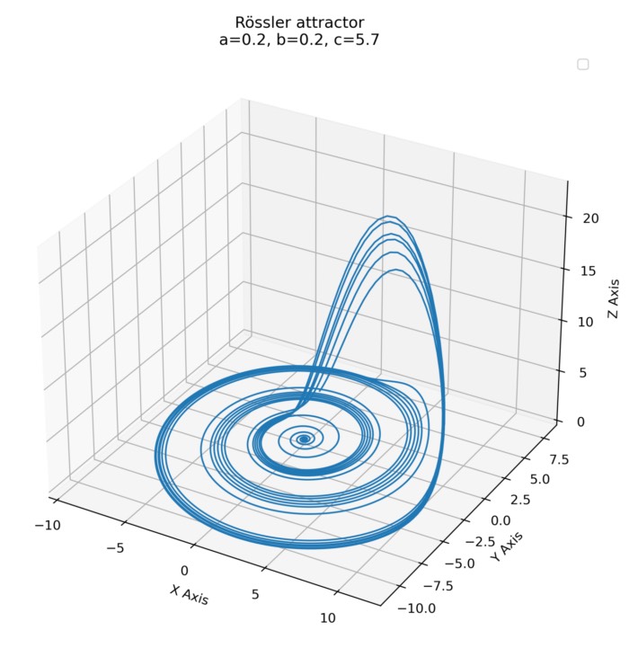
The first of the resulting plots shows the five numerical solutions to the Lorenz system. All solutions show chaotic behavior and look quite similar, but they more or less differ in their trajectories. In general, the accuracy of the solution increases with increasing order of the Runge-Kutta method. The solution obtained using RK4 and RK4/5 (solve_ivp) are the most accurate.

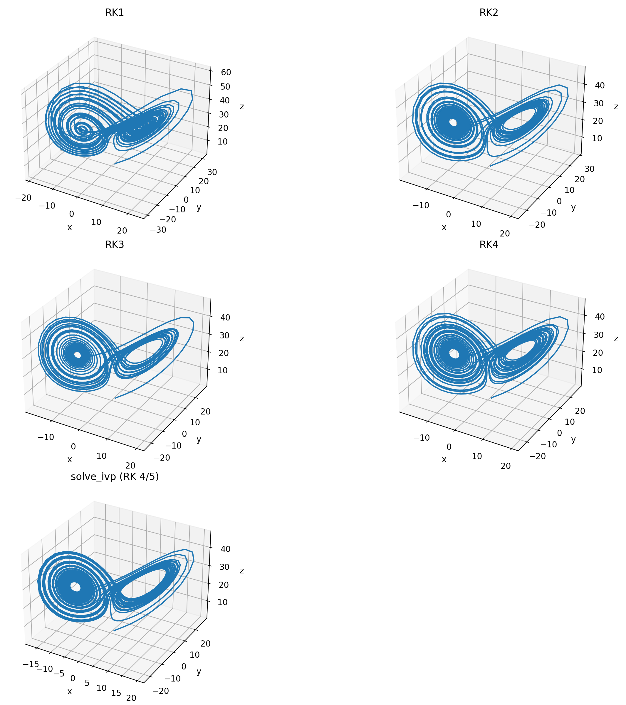The five numerical solutions to the Lorenz system.

However, it is difficult to assess the accuracy of the solutions by just looking at the trajectories. Many physical systems have conserved quantities such as energy. Energy often presents as a quadratic term in the variables of the system. In the Lorenz equations, we do not have a direct representation of physical energy, but we can define a equation, that serves to provide an energy-like measure, which can be useful for numerical studies of the system:

\[E = \frac{x^2}{2} + y^2 + z^2 - z\]

This equation is the sum of quadratic and linear terms of each of the state variables $x$, $y$, and $z$, which is a common form for energy in many physics problems. The defined metric has the advantage of being easily computable and giving a scalar quantity that can be tracked over time, enabling the observation of the system’s behavior under different integration schemes. However, it is essential to note that the Lorenz system does not directly model a physical system where energy is conserved. Thus, the “Lorenz energy” $E$ is an indicative measure and does not have the same strict physical interpretation as energy in physics.

In the Python code, we calculate $E$ for each time step and method. The method that “conserves” this quantity better would generally be considered more accurate. Solutions, that show minimal fluctuations, i.e., oscillations suggest better energy conservations, and the according method can be considered more accurate. Magnitude is another parameter to assess the energy plots. A solution with smaller overall energy deviations from the initial value indicates better energy conservation. You can also assess long-term trends in the energy plots. If the energy consistently increases or decreases over time, it may indicate a deviation from energy conservation.

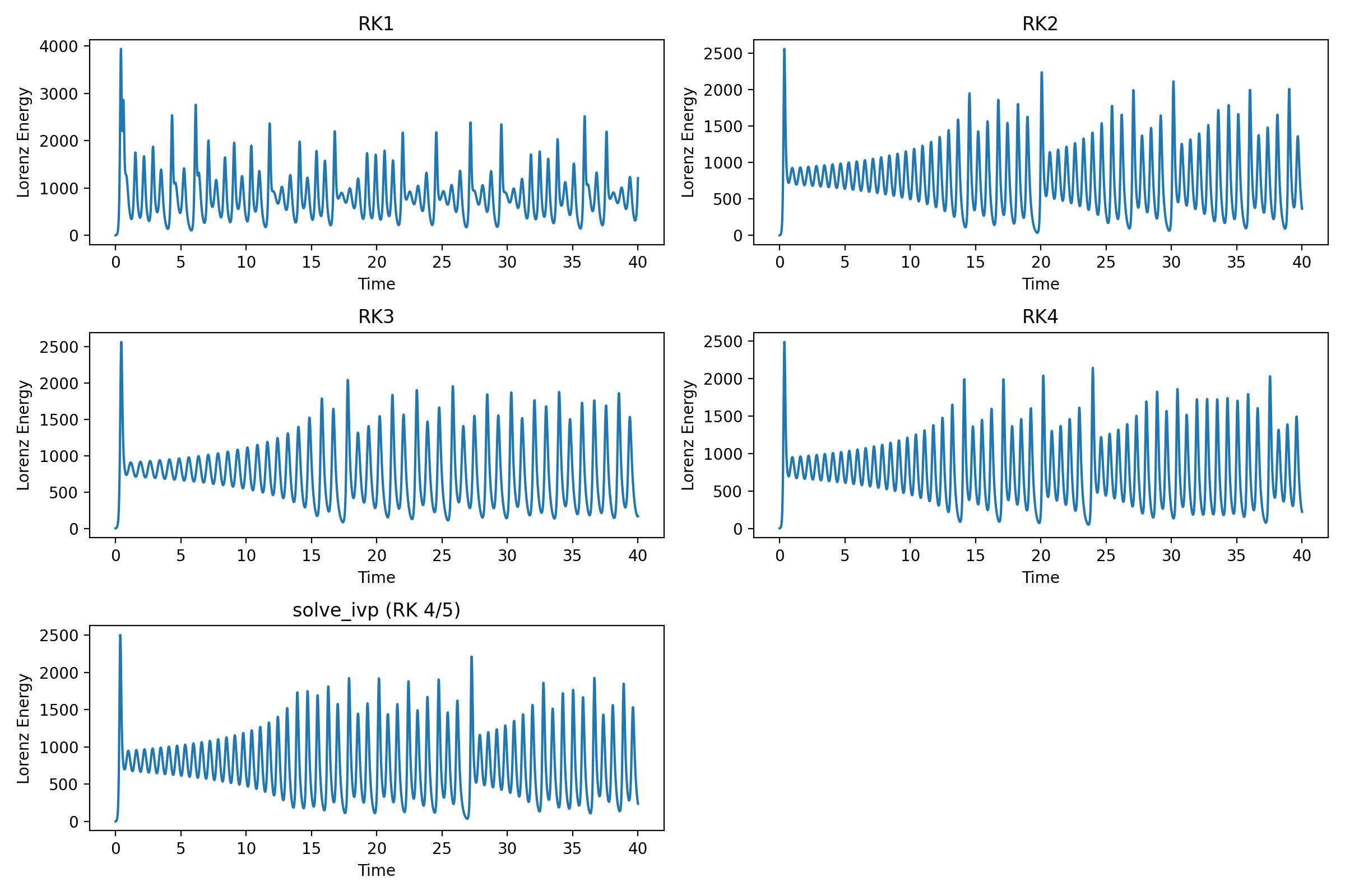The Lorenz energy for the five numerical solutions.

Another approach to assess the accuracy of the solution is the observation of their long-term behavior. For chaotic systems like the Lorenz system, the long-term behavior is of special interest. You could run the simulation for a longer time and see which method’s solution exhibits the expected long-term behavior, such as remaining bounded or demonstrating sensitivity to initial conditions.

Conclusion

We have explored the dynamics of the Lorenz system, a non-linear and chaotic system, using the Runge-Kutta methods. Through numerical integration, we have gained insights into the system’s behavior, where small changes in initial conditions can lead to significant variations in the outcomes (“butterfly effect”). By assessing a custom defined metric, we have evaluated the performance of the numerical integrators. The Runge-Kutta methods provide powerful tools for simulating complex systems like the Lorenz system, enabling us to gain insights into their behavior and dynamics. By leveraging numerical integrators, we can study and understand chaotic systems that defy analytical solutions.

The entire code used in this post is available in this GitHub repositoryꜛ.

If you have any questions or suggestions, feel free to leave a comment below.

If you want to see more RK examples, check out my next post on simulating the orbits of artificial satellites using the Runge-Kutta methods.