FitzHugh-Nagumo model

In the previous post, we analyzed the dynamics of Van der Pol oscillator by using phase plane analysis. In this post, we will see, that this oscillator can be considered as a special case of another dynamical system, the FitzHugh-Nagumo model. The FitzHugh-Nagumo model is a simplified model used to describe the dynamics of the action potential in neurons. With a few modifications of the Van der Pol equations we can obtain the model’s ODE system. By again using phase plane analysis, we can then investigate how the dynamics of the system changes under these modifications.

Derivation of the model

The FitzHugh-Nagumo model is a two-dimensional system of ordinary differential equations (ODEs) that describes the dynamics of the action potential in neurons, i.e., their firing of voltage spikes or pulses. The model was introduced by Richard FitzHugh in 1961 and later modified by J. Nagumo, S. Arimoto, and S. Yoshizawa in 1962. The model is a simplification of the Hodgkin-Huxley model, which is a more complex system of ODEs that describes the dynamics of the action potential in neurons in greater detail.

Let’s consider the Van der Pol oscillator from our previous post:

\[\begin{align} \ddot{x} - \mu (1-x^{2})\dot{x}+x&=0 \end{align}\]

Using the Liénard transformation $y=x-x^{3}/3-{\dot {x}}/\mu$, the oscillator can be transformed into a two-dimensional system of ODEs:

\[\begin{align} \dot{x} &= \mu \left(x-{\tfrac {1}{3}}x^{3}-y\right) \\ \dot{y} &= {\frac {1}{\mu }}x \end{align}\]

In order to make the transition from classical mechanics to a model for the action potential in neurons, we rename the system’s variables accordingly. We rename the state variables $x$ and $y$ to $v$ and $w$, which represent the membrane potential and the recovery variable, respectively:

\[\begin{align} \dot{v} &= \mu(v-\tfrac {1}{3}v^{3}-w) \\ \dot{w} &= \frac{1}{\mu}v \end{align}\]

From the phase plane analysis we know that the Van der Pol oscillator exhibits a stable limit cycle, which is a closed trajectory in the phase space, and has an unstable fixed point in the origin, where the system’s nullclines intersect. Around this fixed point, the system is unstable with a spiral sink behavior, converging to limit cycle.

In order to gain some more control over this fixed point and increasing flexibility over the system’s dynamics, we adjust the ODE system to allow the fixed point to be either a stabile or unstable one, depending on the parameters. This involves altering the system in such a way that the $\dot{w}=0$ nullcline gets tilted. We achieve this by incorporating two additional terms into the $\dot{w}$ equation and introducing a new term to the $\dot{v}$ equation:

\[\begin{align} \dot{v} &= \mu(v-{\tfrac {1}{3}}v^{3}-w + I_\text{ext}) \label{eq:1} \\ \dot{w} &= \frac{1}{\mu}(v + a -b w) \label{eq:2} \end{align}\]

These are the equations of the FitzHugh-Nagumo model. The newly introduced term $I_\text{ext}$ in the $\dot{v}$ equation represents the effect of an external current on the membrane potential $v$. In order to maintain the units of the membrane potential in volts, we should have added $I_{ext}R$ instead of just $I_{ext}$, with $R$ being the membrane resistance. However, we will keep it simple and set $R=1$ and neglect it in the following. The term $a$ in the $\dot{w}$ equation represents the effect of a constant input current on the recovery variable $w$. The term $b w$ represents the effect of the recovery variable $w$ on itself. By setting the newly added parameters to zero, we can recover the original Van der Pol oscillator, making it a special case of the FitzHugh-Nagumo model.

The FitzHugh-Nagumo model is called excitability model as the added external current term, $I_{\text{ext}}$, can trigger the system to generate action potentials. The model exhibits excitability as it requires the external input to generate action potentials. Thus, the FitzHugh-Nagumo model is way more biologically plausible and comparable to the natural behavior of neurons than the Van der Pol oscillator, as we can trigger system responses depending on external inputs. The Van der Pol oscillator, in contrast, is a relaxation oscillator and exhibits oscillations without external input.

Alternative derivations

In the literature, one can find different derivation of the FitzHugh-Nagumo model, which lead to slightly different ODE systems.

In his 1961 publicationꜛ, FitzHugh started with the same differential equation of the Van der Pol oscillator as we did above. However, he used a slightly different Liénard transformation, $y=-x+x^{3}/3+{\dot {x}}/\mu$, which alters the signs of some terms in the transformed system:

\[\begin{align} \dot{v} &= \mu(v+{\tfrac {1}{3}}v^{3}+w + I_\text{ext}) \\ \dot{w} &= - \frac{1}{\mu}(v - a +b w) \end{align}\]

In his 1969 publicationꜛ, FitzHugh started with a different differential equation,

\[\begin{align} \ddot{x} - (1-x^{2})\dot{x}+\phi x&=0 \end{align}\]

applies yet another variant of the Liénard transformation, $y=x-x^{3}/3-{\dot {x}}$, and obtains the following system of ODEs:

\[\begin{align} \dot{v} &= v-{\tfrac {1}{3}}v^{3}-w + I_\text{ext} \\ \dot{w} &= \phi(v + a -b w) \end{align}\]

Both, Scholarpediaꜛ and Wikipediaꜛ seem to follow the derivation from the 1969 publication (in the Wikipedia version, $\mu$ is substituted by $\frac{1}{\tau}$ with $\tau$ being some time constant, that is not further explained).

Gerstner et al. (2014)ꜛ use yet another variant of the model (their Eq. (4.11)), which is derived from the Hodgkin-Huxley model:

\[\begin{align} F(u,w) &= u-{1\over 3}u^{3}-w \\ {G}(u,w) &=b_{0}+b_{1}\,u-w \end{align}\]

Here, one could identify $F(u,w)$ as $\dot{v}$ and $G(u,w)$ as $\dot{w}$ with $u=v$ as well as $b_{0}$ as our $a$ and $b_{1}$ as our $b$. However, why we would then have $b v$ instead of $b w$ remains unclear.

Nagumo et al. (1962)ꜛ used yet another variant,

\[\begin{align} J &= \frac{1}{\mu} \dot{v} -w - (u-\frac{v^3}{3}) \\ \mu \dot{w} + bw &= a-v \end{align}\]

which, by setting $J=0$, yields to:

\[\begin{align} \dot{v} &= \mu(w-\frac{1}{3} v^3 + u) \\ \dot{w} &= \frac{1}{\mu}(v - bw +a) \end{align}\]

These equations share the same structure as the ones from FitzHugh (1961), but with different signs.

Overall, it seems that the FitzHugh-Nagumo model can be derived in different ways, depending on the starting equation used for the Van der Pol oscillator and the Liénard transformation applied. Since some sources do not provide the derivation, it is not always clear how the model was obtained. We will continue with the model as derived in Eq. ($\ref{eq:1}$) and ($\ref{eq:2}$).

Nullclines

As we have learned in the previous posts, the nullclines of a dynamical system are the curves in the phase plane where the derivatives of the state variables are zero. Nullcline provide important information about the system’s dynamics, such as the location of fixed points and the direction of the flow in the phase space. To derive the nullclines of the FitzHugh-Nagumo model, we set the derivatives of the state variables to zero and solve for the other state variable.

Let’s start with Eq. ($\ref{eq:1}$) and calculate $\dot{v}$-nullcline by setting $\dot{v}=0$:

\[\begin{align} & \dot{v} = \mu(v-{\tfrac {1}{3}}v^{3}-w + I_\text{ext}) \stackrel{!}{=} 0 \notag \\ \Leftrightarrow & \; w = v-{\tfrac {1}{3}}v^{3} + I_\text{ext} \end{align}\]

We do the same for Eq. ($\ref{eq:2}$) to calculate the $\dot{w}$-nullcline:

\[\begin{align} & \; \dot{w} = \frac{1}{\mu}(v + a -b w) \stackrel{!}{=} 0 \notag \\ \Leftrightarrow & \; w = \frac{1}{b}(v + a) \end{align}\]

Recall our initial motivation for introducing the additional terms in the Van der Pol equations: We wanted to make the fixed point of the system stable by tilting the $\dot{w}$-nullcline (former $\dot{v}$-nullcline). And indeed, the additional terms have the effect of tilting the $\dot{w}$-nullcline with slope $1/b$ and intercept $a/b$. The $\dot{v}$-nullcline is again a cubic curve. The intersection of the two nullclines is the fixed point of the system.

Python code

To study the dynamics of the FitzHugh-Nagumo model, we can reutilize the Python code from the previous post and modify it accordingly:

import numpy as np
import matplotlib.pyplot as plt
from scipy.integrate import solve_ivp
plt.rcParams.update({'font.size': 14})
import os
if not os.path.exists('figures'):
    os.makedirs('figures')

# define the FitzHugh-Nagumo model:
def fitzhugh_nagumo(t, z, mu, a, b, I_ext):
    v, w = z
    dvdt = mu * (v - (v**3) / 3 - w + I_ext)
    dwdt = (1 / mu) * (v + a - b * w)
    return [dvdt, dwdt]

# define the nullclines:
def v_nullcline(v, I_ext):
    return v - (v**3) / 3 + I_ext
def w_nullcline(v, a, b):
    return (1 / b) * (v + a)

# set time span:
eval_time   = 100
t_iteration = 1000
t_span = [0, eval_time]
t_eval = np.linspace(*t_span, t_iteration)

# set initial conditions:
z0 = [-1, -0.8]
mu = 2.0
a = 0.7
b = 0.8
I_ext = 0.25

# calculate the vector field:
mgrid_size = 3
x, y = np.meshgrid(np.linspace(-mgrid_size, mgrid_size, 15), 
                   np.linspace(-mgrid_size, mgrid_size, 15))
u = mu * (x - (x**3)/3 - y + I_ext)
v = (1/mu) * (x + a - b * y)

# calculating the trajectory for the Van der Pol oscillator:
sol = solve_ivp(fitzhugh_nagumo, t_span, z0, args=(mu, a, b, I_ext), t_eval=t_eval)

# define the x-array for the nullclines:
x_null = np.arange(-mgrid_size,mgrid_size,0.001)

# plot vector field and trajectory:
plt.figure(figsize=(6, 6))
plt.clf()
# plot the streamline plot colored by the speed of the flow:
speed = np.sqrt(u**2 + v**2)
plt.streamplot(x, y, u, v, color=speed, cmap='cool', density=2.0)
plt.plot(x_null, v_nullcline(x_null, I_ext), '.', c="darkturquoise", markersize=2)
plt.plot(x_null, w_nullcline(x_null, a, b), '.', c="darkturquoise", markersize=2)
plt.plot(sol.y[0], sol.y[1], 'r-', lw=3, label=f'Trajectory, $z_0$={z0}')
# indicate start point:
plt.plot(sol.y[0][0], sol.y[1][0], 'bo', label='start point', alpha=0.75, markersize=7)
plt.plot(sol.y[0][-1], sol.y[1][-1], 'o', c="yellow", label='end point', alpha=0.75, markersize=7)
# indicate the direction of the trajectory's last point with an arrow:
plt.title(f'phase plane plot: FitzHugh-Nagumo model\na: {a}, b: {b}, $\mu$: {mu}, $I_$: {I_ext}')
plt.xlabel('v')
plt.ylabel('w')
plt.legend(loc='lower right', fontsize=12.5) 
plt.gca().spines['top'].set_visible(False)
plt.gca().spines['right'].set_visible(False)
plt.gca().spines['bottom'].set_visible(False)
plt.gca().spines['left'].set_visible(False)
#plt.xlim(-mgrid_size, mgrid_size)
plt.ylim(-mgrid_size, mgrid_size)
plt.tight_layout()
plt.show()

# plot v over time to visualize the voltage curve:
plt.figure(figsize=(8, 5))
plt.plot(sol.t, sol.y[0], 'b-', lw=2, label='Voltage $v(t)$')
plt.title(f'voltage curve: FitzHugh-Nagumo model\na: {a}, b: {b}, $\mu$: {mu}, $I_$: {I_ext}')
plt.xlabel('Time')
plt.ylabel('Voltage $v$')
plt.legend(loc='best', fontsize=12.5)
plt.grid(True)
ax = plt.gca()
ax.spines['top'].set_visible(False)
ax.spines['right'].set_visible(False)
ax.spines['bottom'].set_visible(False)
ax.spines['left'].set_visible(False)
plt.tight_layout()
plt.show()

Note, that we have added an additional plot of the voltage curve $v(t)$ to visualize the spiking behavior of the simulated neuron. The entire code can be found in this Github repositoryꜛ.

Simulating an action potential

Before we start, let’s briefly recap the phases of an action potential, that we have already discussed in the post on the Integrate and Fire model:

Shape of a typical action potential. Source: Wikimedia Commonsꜛ (license: CC BY-SA 3.0; modified)

An action potential is a rapid change in the membrane potential of a neuron that allows it to communicate with other neurons. It is evoked when an external stimulus reaches a certain voltage threshold, and consists of three main phases: depolarization, repolarization, and hyperpolarization. The depolarization phase is characterized by a rapid increase in the membrane potential due to the opening of voltage-gated sodium channels and a subsequent influx of sodium ions. This phase is followed by repolarization, where sodium channels start to close and voltage-gated potassium channels open, allowing potassium to exit the neuron and bring the membrane potential back toward the resting level. Hyperpolarization occurs as potassium channels close slowly, causing the membrane potential to become temporarily more negative than the resting potential. This phase is associated with the relative refractory period, during which the neuron requires a stronger stimulus to fire another action potential. The absolute refractory period spans from the onset of depolarization to the end of repolarization, during which the neuron cannot initiate another action potential regardless of stimulus strength. After the hyperpolarization phase, the neuron returns to its resting potential, and the cycle can begin again.

Let’s check whether the FitzHugh-Nagumo model can reproduce these phases. We will simulate the model for different initial conditions and external currents and observe the resulting trajectories in the phase plane. We will also plot the voltage curve $v(t)$ to visualize the action potentials generated by the model.

Setting the initial condition $(v_0, w_0)$ to $(-1.0, -0.8)$ (which corresponds to the z0 variable in the Python code), $a$ to $0.7$, $b$ to $0.8$, and $\mu=2$, and applying an external current of $I_{\text{ext}}=0.25$, we obtain the following phase plane plot and voltage curve:

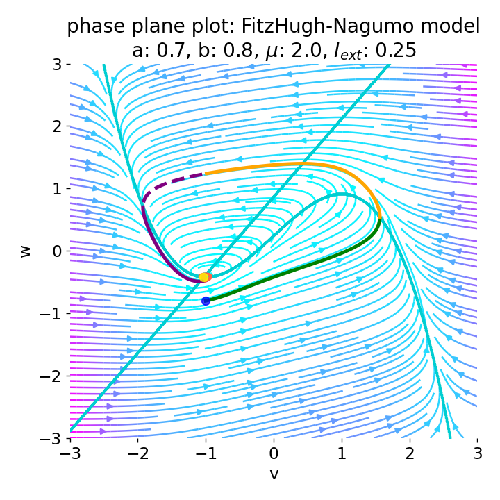
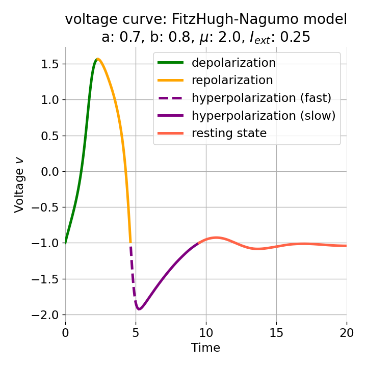Left: Phase plane plot of the FitzHugh-Nagumo model for initial condition $z_0=(-1.0, -0.8)$ and $\mu=2$, $a=0.7$, and $b=0.8$. Nullclines are plotted in cyan, and the vector field is represented by streamlines. Starting and end point of the trajectory are indicated by blue and yellow dots, respectively. Parts of the trajectory are color-coded according different phases of the simulated action potential (depolarization, repolarization, hyperpolarization). Right: Corresponding voltage curve $x(t)$.

With the chosen set of parameters, the model is indeed able to simulate a single action potential and its different phases. To identify the phases, parts of the trajectory and voltage curve are color-coded according to the different phases of the action potential. The voltage curve starts in the depolarization phase (green), where the membrane potential increases rapidly. In the phase plane plot, we can identify this phase being the part of the trajectory, which starts at the initial condition (blue dot) and follows the streamlines towards the $\dot{v}$-nullcline. Once the nullcline is reached, the trajectory has for a short period of time almost just a vertical $w$-component and then follows the streamlines into negative $v$-direction with a relative low $w$-component. This part of the trajectory can be identified as the repolarization phase (yellow) in the voltage curve. However, when the voltage curve passes $v=\sim-1$ (considered as the level of the resting potential, red), the actual hyperpolarization phase (purple) starts. This phase can be further subdivided into a fast (dashed line) and slow part (straight line). During the fast part, the trajectory in phase space is still on the fast track in negative $v$-direction. During the slow part, the trajectory reaches the left part of the $\dot{v}$-nullcline and drops down to the fixed point (the intersection of the nullclines), again having almost just a vertical $w$-component with only slow changes in the $v$-direction, roughly following the left part of the $\dot{v}$-nullcline. The turning point from fast to slow hyperpolarization overlaps with the voltage curve having its global minimum at around $v=-2$. After the turning point, the trajectory’s $v$-component turns from negative to positive values, indicating the (slow) return to the resting potential.

Both the depolarization phase and the repolarization phase roughly take 2.5 time units (each). The relative refractory period, in contrast, roughly takes 5 time units, which is the time both the depolarization and repolarization phase take together, thus being the slowest phase of the action potential, which is consistent with what is observed in real neurons.

The reason for the observed speed differences in the different phases of the action potential can be explained by the structure of the FitzHugh-Nagumo model. The nonlinear term $-\frac{1}{3}v^3$ in the $\dot{v}$ equation introduces a strong nonlinearity to the $v$-dynamics, allowing for rapid changes in $v$ when $v$ is far from equilibrium. This nonlinearity is absent from the $\dot{w}$ equation, making $w$ dynamics more linear and generally slower. Furthermore, time scale separation is explicitly introduced by $\mu$ and its reciprocal in the equations. Typically, in the FitzHugh-Nagumo model, $\mu$ is chosen such that $v$ evolves on a faster time scale than $w$, representing the fast response of the membrane potential compared to the slower recovery processes modeled by $w$. We have chosen $\mu=2$ in our simulation, which ensures that the $v$-dynamics are faster than the $w$-dynamics.

After the hyperpolarization phase, the trajectory does not completely return to the rest state, but starts a new cycle in our case. This cycle, however, is less pronounced than the first one, reaching lower amplitudes and time intervals, indicating a dampening of the action potential’s intensity over time. This behavior is reflected in the phase plane plot, where the trajectory does indeed not fully return to the equilibrium point, but starts a new, much shorter cycle with reduced dynamical expression compared to the initial one. We will discuss this behavior in more detail in the next section.

Overall, the FitzHugh-Nagumo model is able to simulate the different phases of an action potential and the subsequent refractory periods. The model captures the essential dynamics of the action potential and provides a simple yet effective way to study the behavior of neurons and their firing mechanisms.

Threshold behavior

Note, that the initial condition that I have chosen for $I_{ext}$ seem to be quite arbitrary. I tried to fit the equilibrium point of the system in phase space, however, I missed the exact point and the system started having already some amount of voltage amplitude and being on a dynamic trajectory in the phase plane (you can verify this by setting $I_{ext}=0$ in the previous simulation). The equilibrium point can actually be calculated exactly by finding the intersection of the nullclines. In the Python code, this can be done by adding the following lines:

v_range = np.linspace(-3.5, 3.5, 400)
v_nullcline_w = v_nullcline(v_range, I_ext)
w_nullcline_v = w_nullcline(v_range, a, b)
intersection = np.argmin(np.abs(v_nullcline_w - w_nullcline_v))
# reset z0 to the intersection point:
z0 = [v_range[intersection], w_nullcline_v[intersection]]
print(z0)

[-1.2017543859649122, -0.6271929824561404]

Updating the initial condition to the intersection point, we obtain the following phase plane plot and voltage curve:

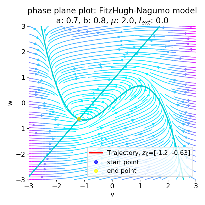
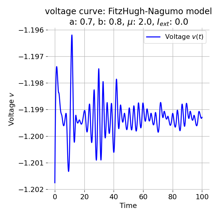Phase plane plot (left) and voltage curve (right) of the FitzHugh-Nagumo model for initial condition matching the equilibrium point in phase space, i.e., the intersection of the nullclines (here, roughly, $z_0=(-1.20, -0.63)$. All other parameters are the same as in the previous simulation except for $I_{ext}$, which is now set to 0. No action potential is generated.

As we see, no action potential is generated and the system converges to the resting potential. However, the system is not fully at rest but exhibits small oscillations around the resting potential. In the phase plane plot, the trajectory starts small new cycles each time before reaching the equilibrium point:

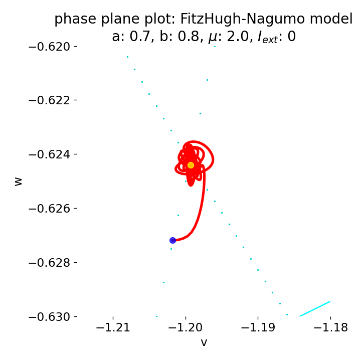
Zoom into the phase plane plot from above. The trajectory starts small new cycles each time before reaching the equilibrium point. Eventually the system will converge to the equilibrium point and remain there, as the system is damped over time. However, I have not determined how long this will take.

This behavior is consistent with what one would expect, as, for the chosen $I_{\text{ext}}$, the intersection of the nullclines becomes a stable fixed point of the system, which converges to a stable limit cycle around this fixed point. The system does not generate an action potential as the trajectory does not generate the necessary dynamics for an action potential to evolve. Instead, the system exhibits low-amplitude oscillations around the resting potential. This can be considered as biophysically plausible, as neurons can exhibit sub-threshold oscillations in the absence of external stimuli.

However, as soon as we add some amount of external current, the equilibrium point will start to move away from its former position and the dynamics of the trajectory will change. For example, setting $I_{\text{ext}}=0.03$, the system becomes able to generate an action potential:

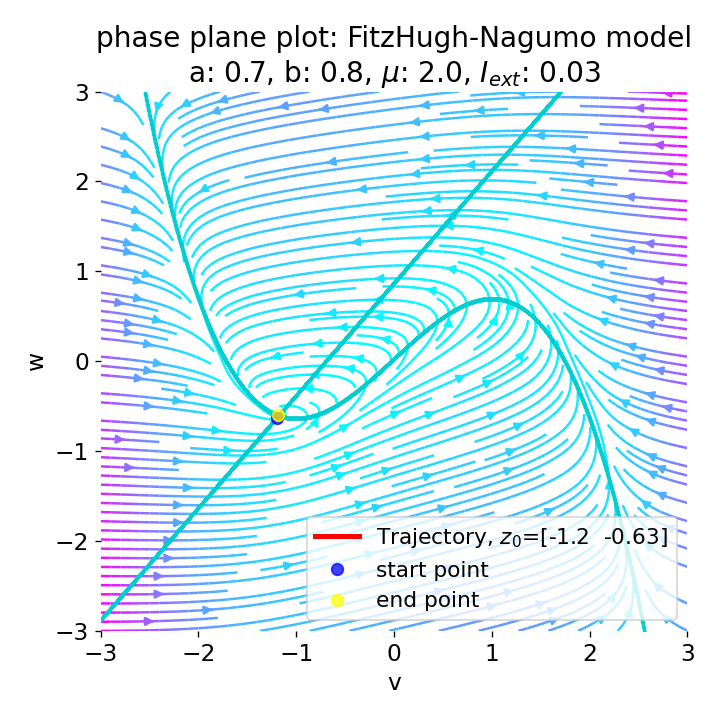
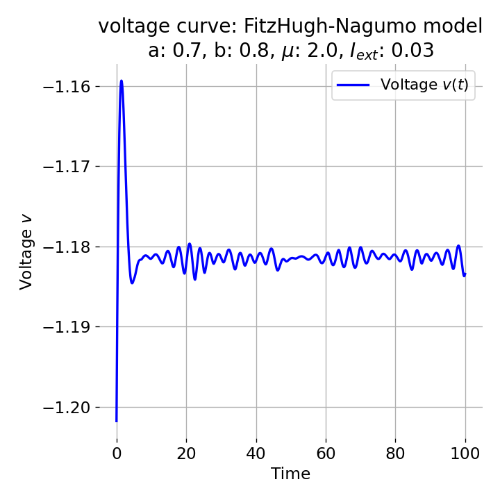Same plots as before, but now for $I_{ext}=0.03$. A pronounced action potential is generated followed by low-amplitude voltage oscillations.

The increase of the external current slightly shifts the $\dot{v}$-nullcline to the right, relocating the fixed point, that is now located at

[-1.1842105263157894, -0.6052631578947367]

The previously chosen initial condition is now clearly located away from the new equilibrium point and a limit cycle with more pronounced dynamics can evolve. The higher the external current, the higher the amplitude of the action potential, as the trajectory becomes more pronounced in the phase plane:

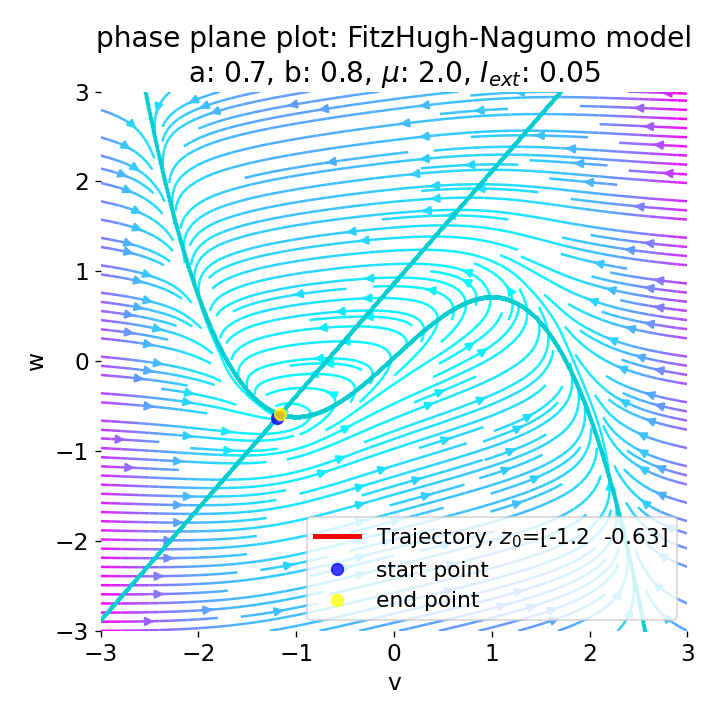
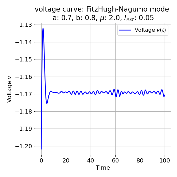
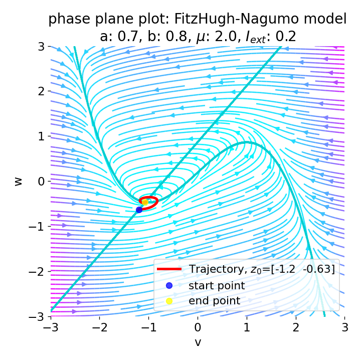
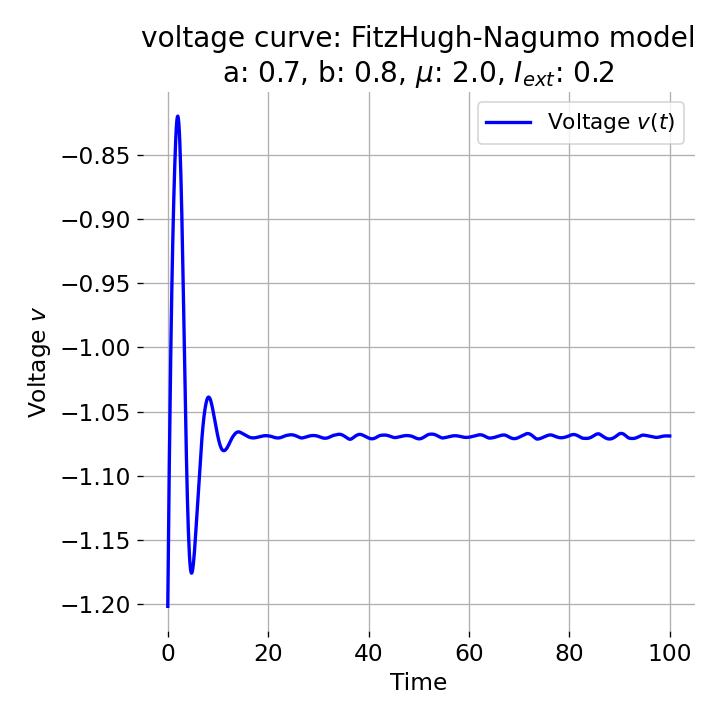Same plots as before, but now for $I_{ext}=0.05$ and $0.2$. The higher the external current, the higher the amplitude of the action potential.

However, an action potential is not necessarily generated for every increase of the external current. The increase must be high enough to shift the equilibrium point sufficiently away from the initial condition. An external current of, e.g., $I_{\text{ext}}=0.005$ is not sufficient to significantly shift the equilibrium point and to trigger an action potential:

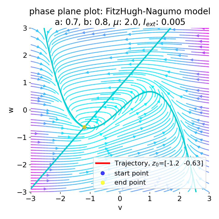
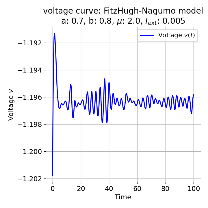Same plots as before, but now for $I_{ext}=0.005$. Indeed, we can identify an initial peak in the voltage curve, but the system does not generate an action potential.

The corresponding equilibrium point is still located at

[-1.2017543859649122, -0.6271929824561404]

Thus, a certain amount of external current is required to trigger the action potential, which is consistent with the behavior of real neurons, where a certain threshold potential must be reached to generate the action potential.

Note, that while we increased the external current, also the resting potential of the system increased. The more we increase the current, the more the $\dot{v}$-nullcline shifts to the right and the more the fixed point (equilibrium point) is located at a higher voltage level. The system maintains the new resting potential since the external current is applied constantly for the entire simulation time. As soon as the current would be removed, the system would return to its initial resting potential.

Spike trains

So far, we were able to simulate a single action potential. However, neurons can generate multiple action potentials in a short period of time, forming so-called spike trains. Spike trains are the fundamental way in which neurons communicate with each other and encode information. They can be regular or irregular, and their timing and frequency can carry important information about the stimulus the neuron is responding to.

In the previous two sections, we have chosen $I_{\text{ext}}$ in such a way, that the intersection of the nullclines became a stable fixed point and the system converged to a stable limit cycle, resulting in the observed single action potential and sub-threshold oscillations of the membrane potential. To simulate a spike train, we need to modify the external current $I_{\text{ext}}$ in such a way that the fixed point becomes unstable. Let’s therefore apply different external currents to the system, keep all other parameters constant, and observe the resulting trajectories in the phase plane

For $I_{\text{ext}}=0.3$, the system generates a pronounced action potential, as described before. After the first pronounced cycle in phase space (which generates the action potential), the system converges to the low-amplitude limit-cycle around the stable fixed point, generating sub-threshold oscillations.

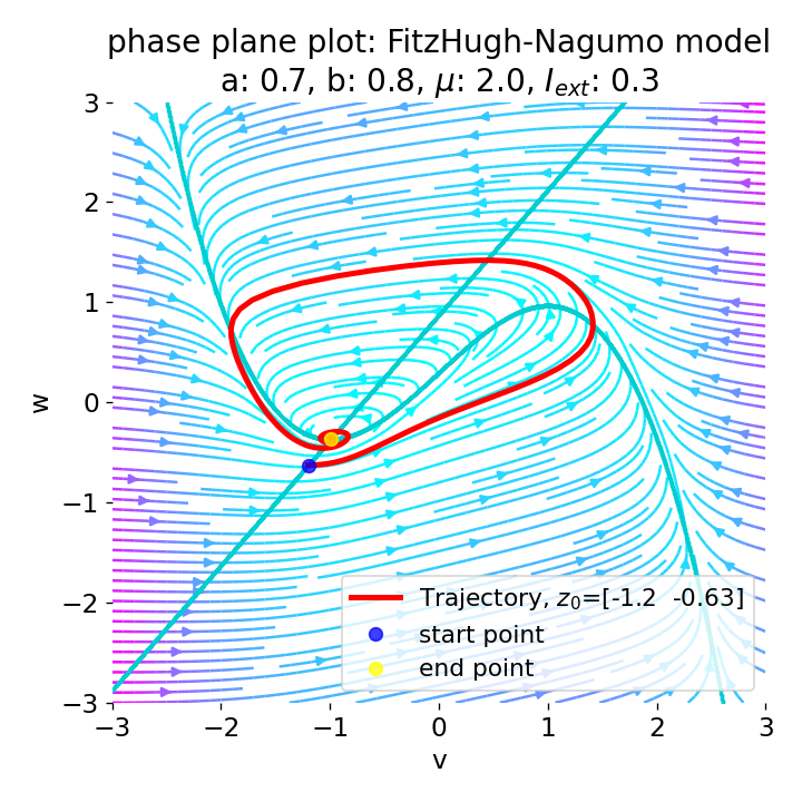
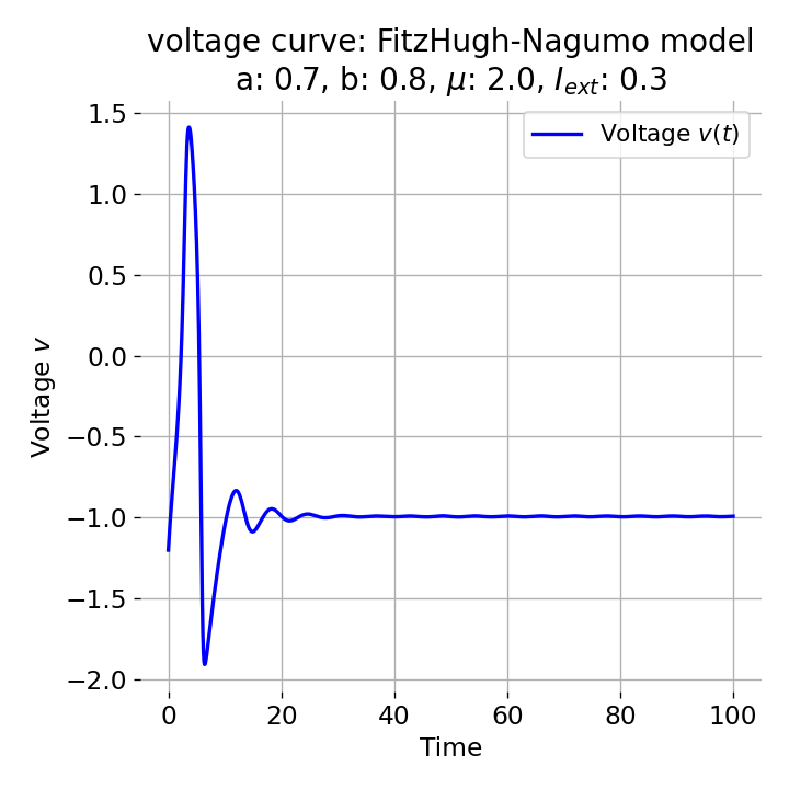Same plots as before, but now for $I_{ext}=0.3$. A pronounced action potential is generated.

For $I_{\text{ext}}=0.4$, the system generates a series of action potentials, forming a spike train. The fixed point has now become unstable and the system converges to a pronounced limit cycle around this fixed point. The first part of the trajectory is a bit elongated due to the large distance between the initial condition and the new fixed point. This results in the first action potential having a higher amplitude than the following ones.

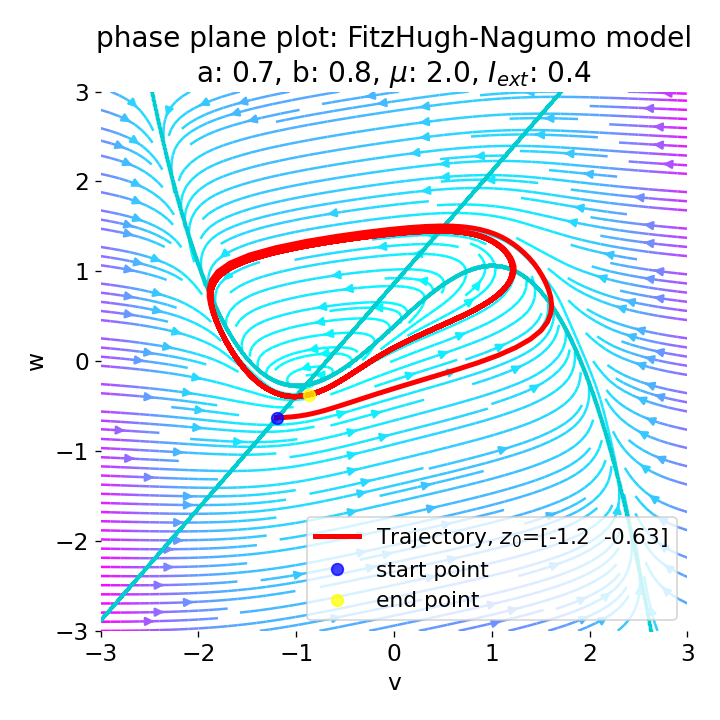
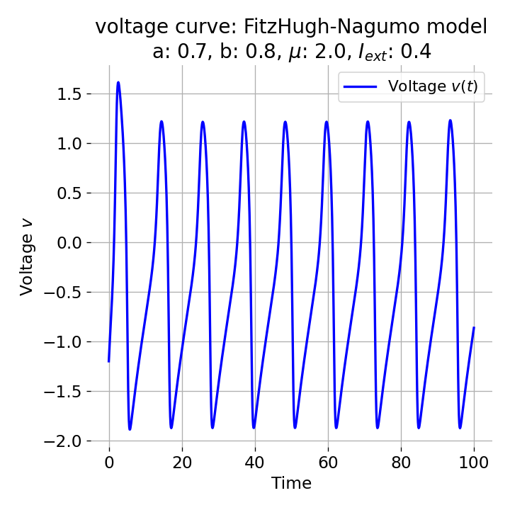Same plots as before, but now for $I_{ext}=0.4$. The system generates a series of action potentials.

The frequency of the action potentials depends on the external current and the resulting dynamics of the system. For $I_{\text{ext}}=0.9$, the system generates a higher frequency of action potentials and thus simulates a neuron that reacts more strongly to the external input and is therefore more excitable.

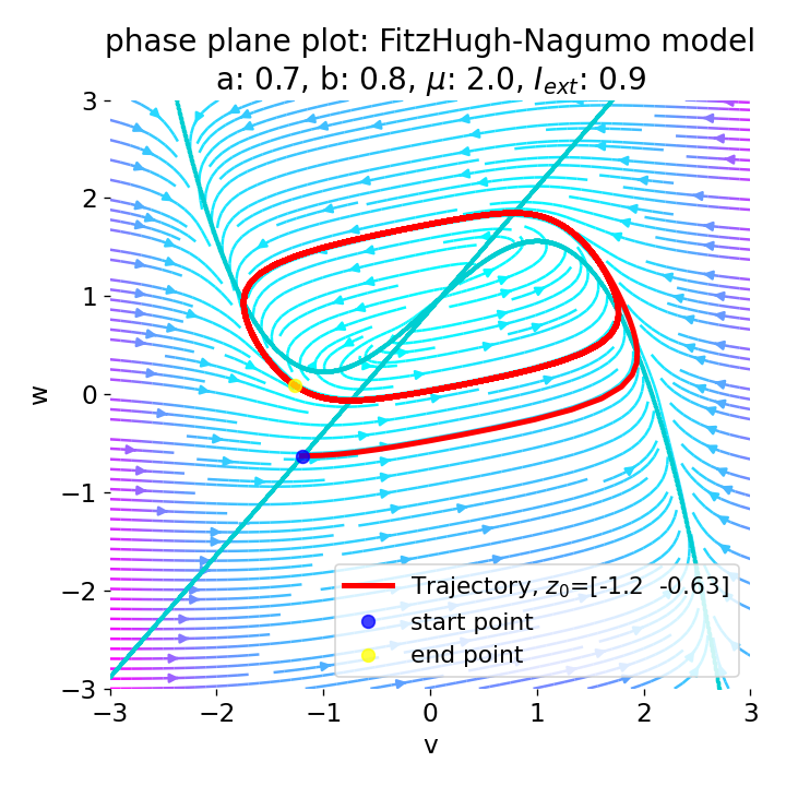
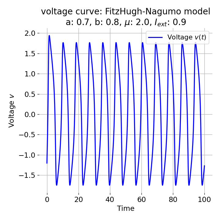Same plots as before, but now for $I_{ext}=0.9$. The frequency of the action potentials increases.

For $I_{\text{ext}}=1.5$, no spike train is generated and we again get a single action potential followed by sub-threshold oscillations. The increase of the external current was too high this time so that the intersection of the nullclines became a stable fixed point again and the system converges to a stable limit cycle around this fixed point. Before reaching this limit cycle, the trajectory has an elongated part due to the large distance between the initial condition and the new fixed point, which results in the single action potential or voltage peak. This is true for any further increase of the external current. One could interpret this behavior as follows: The system is too excited by the external current and the fixed point is shifted too far away from the initial condition. As a result, the oscillations of the system (the spike trains) are blocked by the too high excitation. In biological terms, this phenomenon is known as the excitation block, where repetitive spiking is blocked as the amplitude of the stimulus current increases. The neuron is overstimulated and cannot generate spike trains.

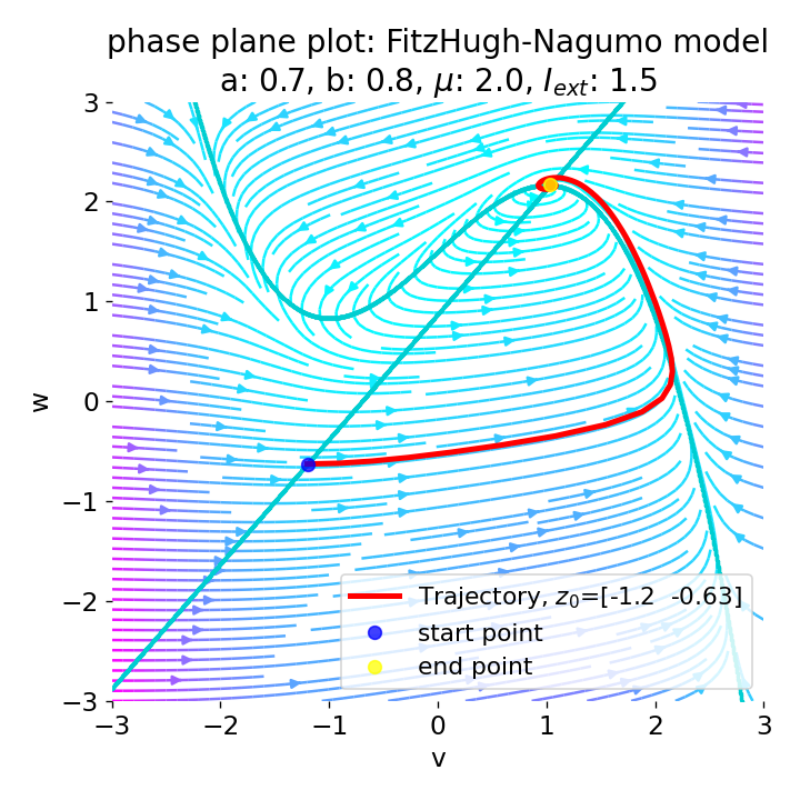
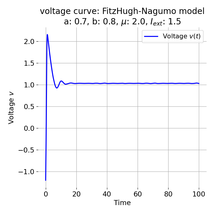Same plots as before, but now for $I_{ext}=1.5$.

In summary, it seems that there is a certain range of external currents that can trigger the generation of spike trains. Outside this range, the system converges to a stable limit cycle around a fixed point and generates either a single action potential or just a low- or high-amplitude voltage peak. In order to further determine this range, let’s have a detailed look at the nullclines and the fixed points for distinct external currents:

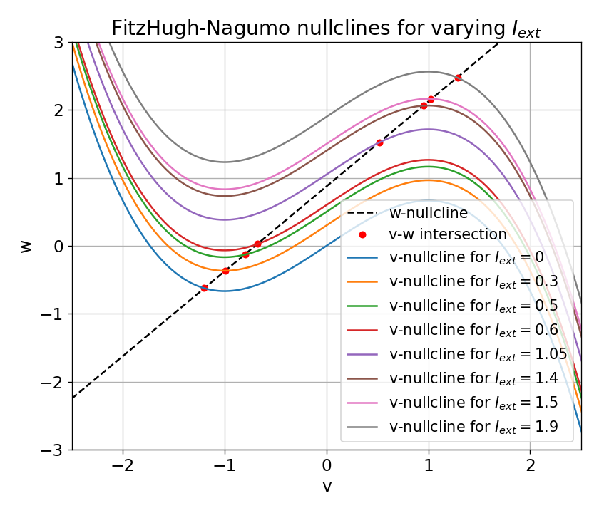Nullclines for distinct external currents: $I_{\text{ext}}=0.0, 0.03, 0.05, 0.3, 0.4, 0.9, 1.5$, and $1.9$. The fixed points at the intersection of the nullclines is indicated by a red dot.

In the plot above, nullclines for distinct external currents are shown. The fixed points at the intersection of the nullclines are indicated by red dots. For $I_{\text{ext}}=0.0$, the fixed point is stable and the system converges to a stable limit cycle around this fixed point. From the previous sections we know that no action potential is generated in this case. By taking a closer look at the plot, we can see that the fixed point is located left to the trough of the $\dot{v}$-nullcline (which is why the system converges to the stable limit cycle).

For $I_{\text{ext}}=0.03$, the fixed point is located almost at the trough of the $\dot{v}$-nullcline, being at the verge of becoming unstable. The system generates a single action potential followed by sub-threshold oscillations as described before. For $I_{\text{ext}}=0.05$, the fixed point is located right to the trough, being unstable. The system converges to a stable limit cycle around this fixed point and generates spike trains. For all other external currents until $I_{\text{ext}}=1.4$ (including), the system generates spike trains (see plot below). All these fixed points are located right to the trough and left to the peak of the $\dot{v}$-nullcline, making them unstable. However, as soon as we exceed the peak to the right, the fixed point becomes stable again and the system converges to a stable limit cycle around this fixed point. This is the case for $I_{\text{ext}}=1.5$ and $I_{\text{ext}}=1.9$.

From these observations, we identify the left trough and the right peak of the $\dot{v}$-nullcline to be critical points in understanding the dynamics of the system. The left and the right part of the N-shaped $\dot{v}$-nullcline are “stable” branches, where the fixed point is stable and the system converges to a stable limit cycle around this fixed point. The middle part is the “unstable” branch, where the fixed point is unstable and the system generates spike trains. This divides the phase plane into two distinct regions:

• outside the trough-peak range: If the fixed point is on the far left or far right stable branches of the $v$-nullcline and outside the trough-peak range, it becomes stable and small perturbations will return to the fixed point without initiating spike trains or a single action potential (or just a low- or high-amplitude voltage peak). This is because the system is pushed back towards the stable branches of the $v$-nullcline, preventing the generation of sustained oscillations.
• within the trough-peak range: If the fixed point lies within the trough-peak range, it becomes unstable and perturbations can lead the system away from the fixed point, across the unstable middle branch, and into spiking behavior. This is because, within this range, the nonlinear dynamics facilitate repetitive excursions around the phase plane that correspond to limit cycles.

Constant oscillations (spike trains) occur when the system’s dynamics force it to repeatedly traverse a path in the phase plane that loops around, typically encompassing parts of both stable branches and the unstable middle branch of the $v$-nullcline. This looping behavior represents the system repeatedly being pushed away from one stable branch, moving through the unstable region, approaching the other stable branch, and then being pulled back, creating a continuous cycle.

To summarize our observations and verify our findings, we apply a ramping external current to the system, starting from $I_{\text{ext}}=0.0$ and increasing it continuously until $I_{\text{ext}}=1.9$:

def fitzhugh_nagumo_time_dependent_ramping(t, z, mu, a, b, 
                                   I_ext_start, I_ext_end, eval_time):
    v, w = z
    # linearly ramp I_ext from I_ext_start to I_ext_end over the time span:
    I_ext = I_ext_start + (I_ext_end - I_ext_start) * (t / eval_time)
    dvdt = mu * (v - (v**3) / 3 - w + I_ext)
    dwdt = (1 / mu) * (v + a - b * w)
    return [dvdt, dwdt]

# set parameters for I_ext ramping:
I_ext_start = 0.0  # Starting value of I_ext
I_ext_end = 1.9    # Ending value of I_ext

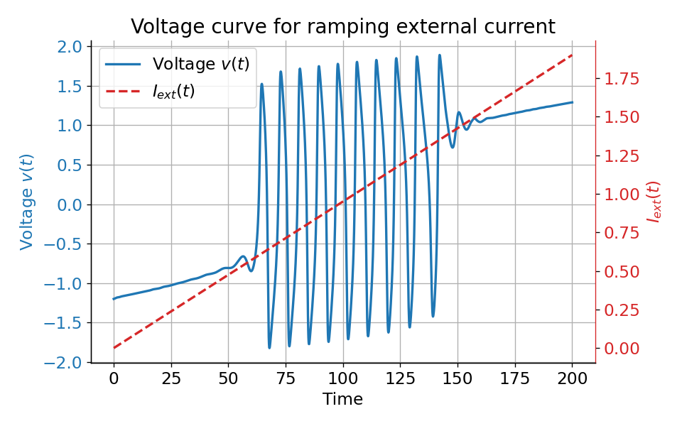Voltage curve $v(t)$ (left y-axis) for a ramping external current (right y-axis) from $I_{\text{ext}}=0.0$ to $I_{\text{ext}}=1.9$. The system generates spike trains for $I_{\text{ext}}=0.05$ to $I_{\text{ext}}=1.4$.

The plot above clearly shows that the system generates spike trains for $I_{\text{ext}}=\sim0.05$ to $I_{\text{ext}}=\sim1.4$, which corresponds to the range where the fixed point is unstable and located within the unstable trough-peak range of the $v$-nullcline. Before and after this range, the system either converges to a stable limit cycle around a fixed point or does not generate any action potentials at all.

Time-dependent external current

Simulating a spike train with a continuous external current is straightforward. However, in reality, neurons receive a variety of inputs from other neurons, which are often not continuous but rather occur in the form of synaptic inputs. Synaptic inputs are brief, transient changes in the membrane potential that are caused by the release of neurotransmitters from other neurons. These inputs can be excitatory or inhibitory, and their timing and frequency can have a significant impact on the firing behavior of the neuron. To simulate the effect of synaptic inputs on the FitzHugh-Nagumo model, we can apply a time-dependent external current to the system. This external current can mimic the effect of excitatory or inhibitory synaptic inputs on the neuron and allow us to study how the neuron responds to different input patterns.

To do so, we redefine the FitzHugh-Nagumo model with a time-dependent external current in such a way, that we can define different time ranges during which the external current is applied:

# define the FitzHugh-Nagumo model with time-dependent (pulsed) I_ext:
def fitzhugh_nagumo_time_dependent_pulse(t, z, mu, a, b, I_ext, pulse_time_ranges):
    v, w = z
    # set I_ext to zero except at pulse_time:
    I_ext_use = 0.0
    # add a pulse during pulse_time_range:
    for pulse_time_range in pulse_time_ranges:
        if (t >= pulse_time_range[0]) and (t <= pulse_time_range[1]):
            I_ext_use = I_ext
    dvdt = mu * (v - (v**3) / 3 - w + I_ext_use)
    dwdt = (1 / mu) * (v + a - b * w)
    return [dvdt, dwdt]

# set time span:
eval_time   = 50
t_iteration = 200

# set parameters for I_ext pulsed:
I_ext = 1.0  # external current during pulse
pulse_time_ranges = [[10,11]]

The remaining parameters are the same as before except for the evaluation time, which is now set to 50 time units. We also reduced the time resolution to 400 iterations to adapt it to the new evaluation time. This means, that, supposing that one time unit corresponds to one second, one second is resolved with eight time steps. When we apply a current pulse of 1 second by setting the pulse_time_ranges, e.g., to [[10,11]], which would correspond to the time span of 1 second, we actually apply a pulse lasting eight time steps. By definition, this is not a delta pulse. Therefore, bear in mind, that a pulse of 1 second in the context of our simulation is not a delta pulse. We can consider it as a short pulse instead.

Let’s evaluate the system with a short pulse external current released at two different time points, $t=9$ and $t=10$:

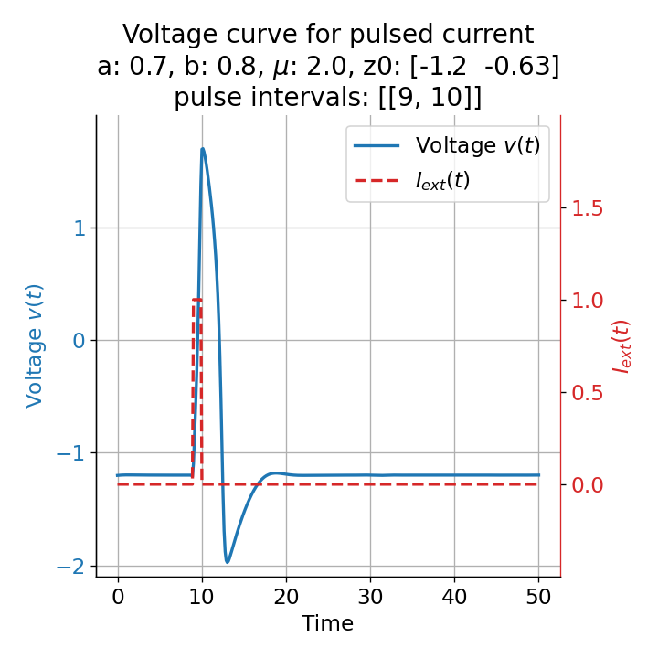
Voltage curves for two short current pulses released at $t=9$ (left) and $t=10$ (right).

For the pulse released at $t=9$, the system generates a single action potential. Even though we applied an external current that was high enough to trigger a spike train when applied continuously (see previous section), the short pulse was not sufficient to generate such multiple action potentials. This is no surprise, as the system’s dynamics are changed only for a short period of time and return to the sub-threshold oscillations after the pulse is over.

When applying the same pulse released at $t=10$, however, no action potential is triggered. Thus, depending on the current location of the trajectory in phase space at the onset of the pulse, the system can either spike or not spike when applying a short pulse. Remember, that before the pulse is applied, the external current is zero and the system exhibits the observed sub-threshold oscillations. This variability in response capability actually highlights another key advantage of the model. Specifically, the model’s ability to simulate sub-threshold oscillations due to diminished and chaotic limit cycle behavior around the stable fixed point introduces another element of randomness. This randomness mirrors the stochastic nature observed in real neurons, where synaptic input timing and frequency crucially influence neuronal firing behavior. Consequently, the system’s differential response to identical pulses, contingent upon input timing, underscores the critical role of synaptic input patterns in determining neuronal activity.

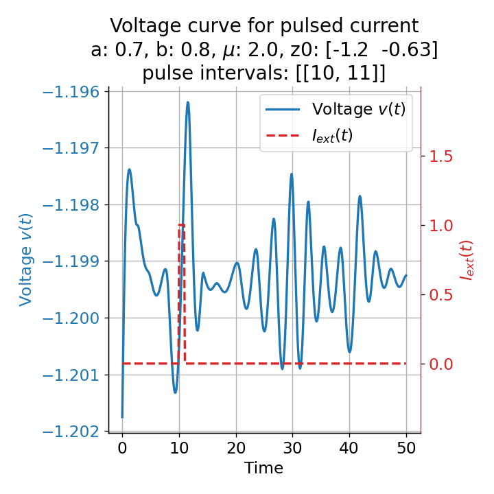
Furthermore, the randomness in the system also affects the absolute amplitude of the action potential. The same short pulse released at different times, e.g., at $t=13$ and, $t=14$, leads to different action potential amplitudes, introducing another randomness factor in the simulation and, thus, a more realistic behavior of the model:

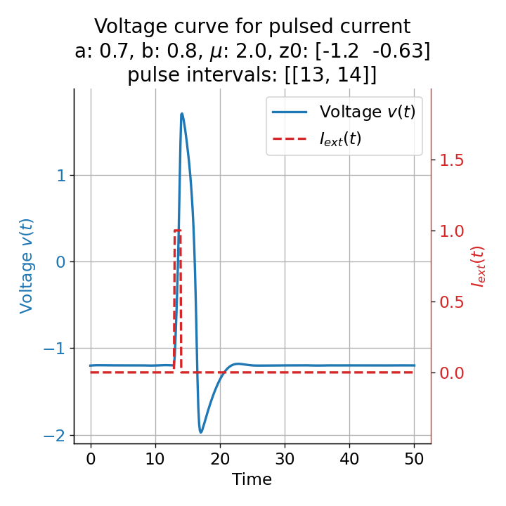
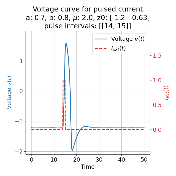Voltage curves for two short current pulses released at $t=13$ (left) and $t=14$ (right). The amplitude of the action potential varies depending on the timing of the pulse with $v_{max}=1.71$ and $v_{max}=1.59$ respectively.

Absolute refractory period

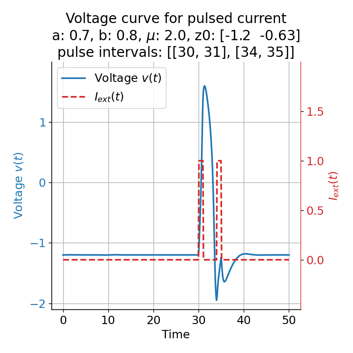
By applying a time-dependent external current, we can now also prove that during the absolute refractory period, the system cannot spike. For example, setting the initial pulse at $t=30$ triggers an action potential. Another pulse anywhere between $t=31$ and $34$ does not trigger a new action potential until $t=35$, where another action potential is triggered. This is an important aspect of the model, as it mimics the absolute refractory period of real neurons, where a neuron cannot spike again during this period. The neuron’s response to external stimuli is thus highly dependent on the timing of the stimuli, which is a crucial aspect of neuronal excitability and spike-generating mechanisms.

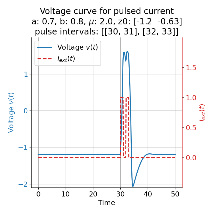
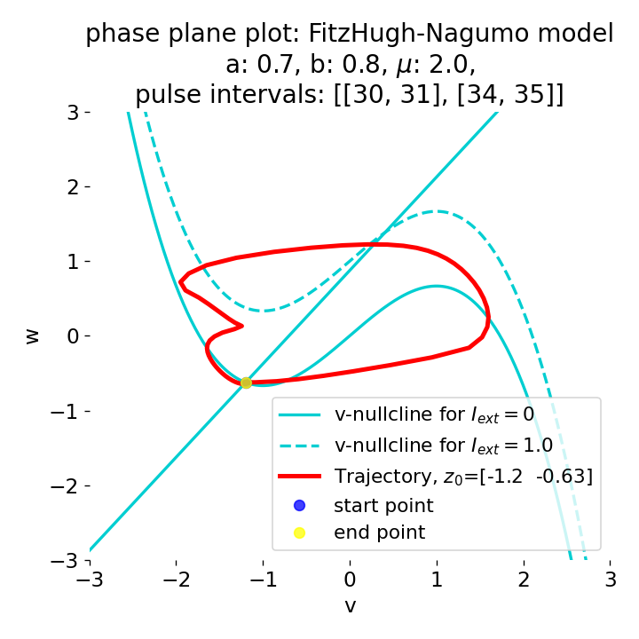
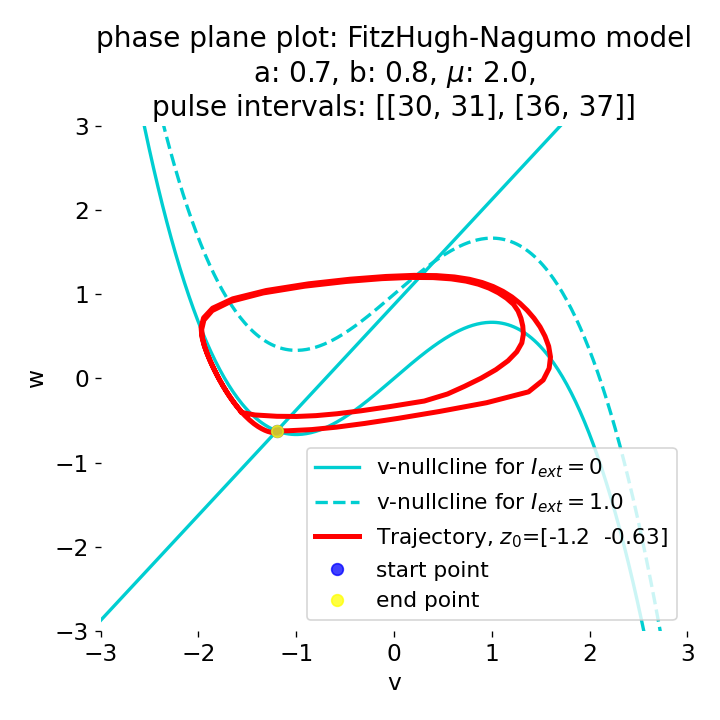
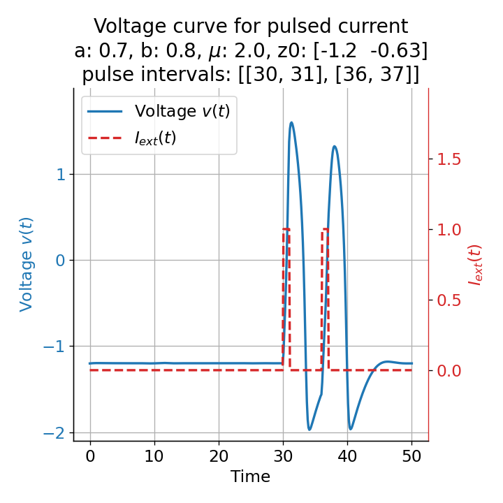Phase plane plots (left) and voltage curves (right) for two short current pulses released in quick succession. In the phase plane plot, two $\dot{v}$-nullclines are plotted, one for each pulse ($I_{\text{ext}}=0.0$ and $1$). Note, that each activation of the current pulse shifts the fixed point of the system at another location (the intersection of the $\dot{v}$ and $\dot{w}$-nullclines). Streamlines are omitted due to the time-dependent nature of the external current. Start and end points of the trajectories are identical as the system starts at $I_{\text{ext}}=0.0$ and ends at $I_{\text{ext}}=0.0$ due to the defined pulse intervals.

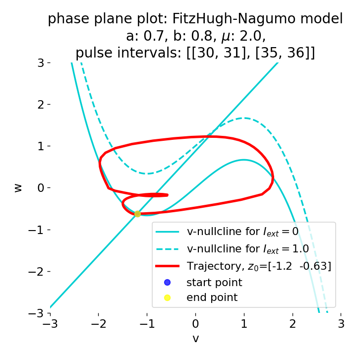
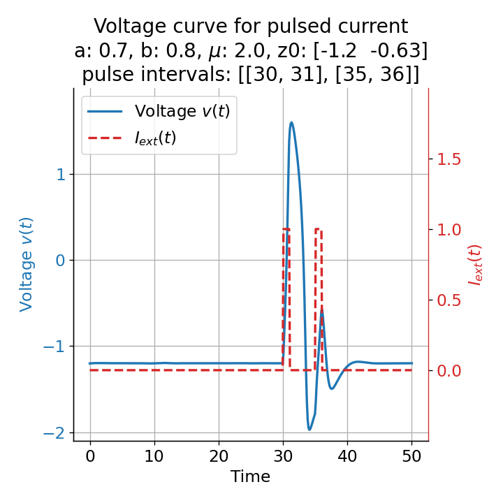
From the phase plane plots above we can extract further details of the dynamics during pulses released during and after the absolute refractory period. For instance, the double-peak that we observe in the voltage curve for a second pulse released at $t=32$ (upper panel) is not due a potentially triggered second action potential that overlaps the first one. Instead, it is caused by a short-time distortion on the depolarizing branch of the trajectory in phase space that does not result into the beginning of another limit cycle. The same is true for the second pulse being release at $t=34$ (upper middle panel). Here, the short-time distortion lays on the hyperpolarizing branch of the trajectory. The distortion is again insufficient to trigger a new limit cycle and, thus, another action potential. This changes when the second pulse is released at $t=35$ (lower middle panel). Here, the system generates a second limit cycle, that is less pronounced than the first one, resulting in a second action potential of lower amplitude. And finally, when the second pulse is released at $t=36$ (lower panel), the system generates a full established second limit cycle, resulting in a second action potential. The amplitude is a bit lower than the first one as the second limit cycle is a bit less pronounced than the first one. Note, that each pulse activation shifts the $\dot{v}$-nullcline a bit further to the right and, thus, the fixed point of the system is also located at another position, resulting in the observed distortions of the trajectories. Also note, that the trajectories in each simulated scenario starts and ends at the same location (the blue and yellow dots overlap each time), as the system starts at $I_{\text{ext}}=0.0$ and ends at $I_{\text{ext}}=0.0$ due to the chosen pulse intervals.

If we apply a longer pulse, the system will spike again continuously. As soon as the external current is removed, the system returns to the resting state as previously assumed:

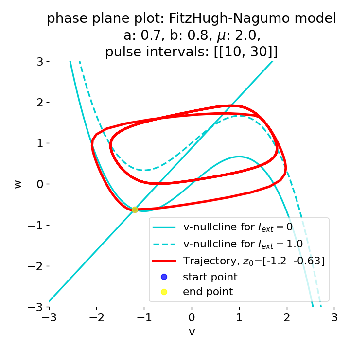
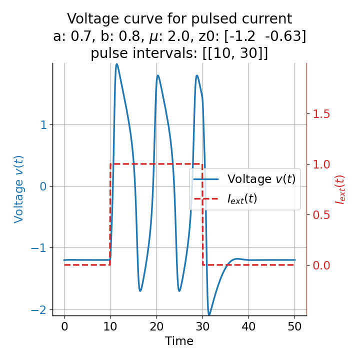Phase plane plots (left) and voltage curves (right) for a long-lasting current pulse ranging from $t=10$ to $t=30$. The system generates spike trains during the pulse and returns to the resting state after the pulse is over.

Abrupt vs. ramped external current

Another important aspect the FitzHugh-Nagumo model is its different response to slowly ramped external currents compared to abruptly increased external currents. During a gradually increasing of the external current (upper panel in plot below), we observe that the resting equilibrium point of the model moves slowly towards the right, with the system’s state transitioning smoothly alongside it, without generating any spikes. In contrast, if the stimulation is increased abruptly (lower panel), even by a smaller magnitude, the system’s trajectory doesn’t move straight to the new equilibrium. Instead, it produces a transient spike. This was the reason why we observed a single action potential for, e.g., $I_{\text{ext}}=0.03$ in the previous sections, where the applied external current was always increased abruptly.

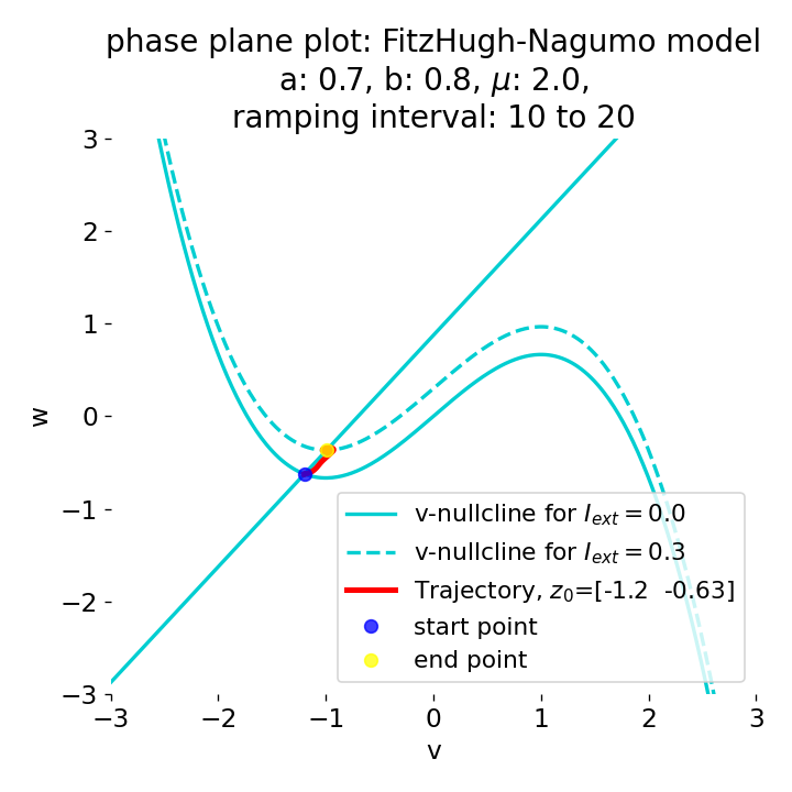
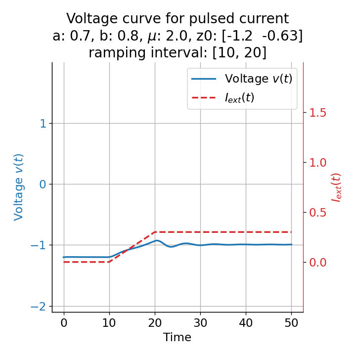
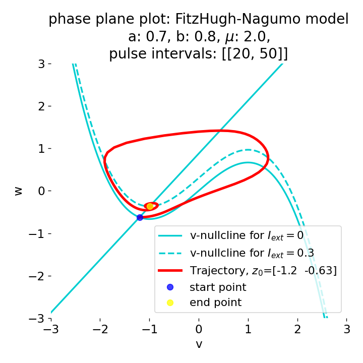
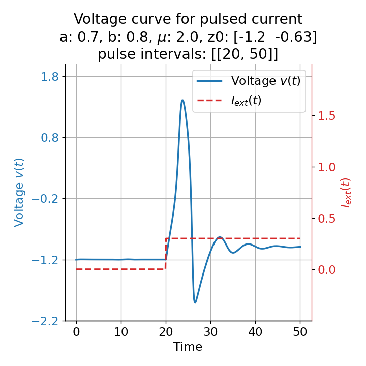Phase plane plots (left) and voltage curves (right) for slowly ramped external current from $I_{\text{ext}}=0.0$ to $I_{\text{ext}}=0.3$ (upper panel) and for an abruptly increased external current from $I_{\text{ext}}=0.0$ to $I_{\text{ext}}=0.3$ (lower panel). In both cases, the final current is reached at $t=30$. The system generates a single action potential for the abruptly increased external current, while no action potential is generated for the slowly ramped external current.

The same is true for external currents, that shift the fixed point into the trough-peak range of the $\dot{v}$-nullcline, i.e., cause the system to generate spike trains. If the external current is increased abruptly, the first action potential of the spike train is a bit higher than the following ones, while in the case of gradually increased external current, all action potentials have the same amplitude (except for the spike(s) that may occur during the ramping period; compare plots below). This is due to the fact that the system has more time to adjust to the new equilibrium point in the case of the slowly ramped external current.

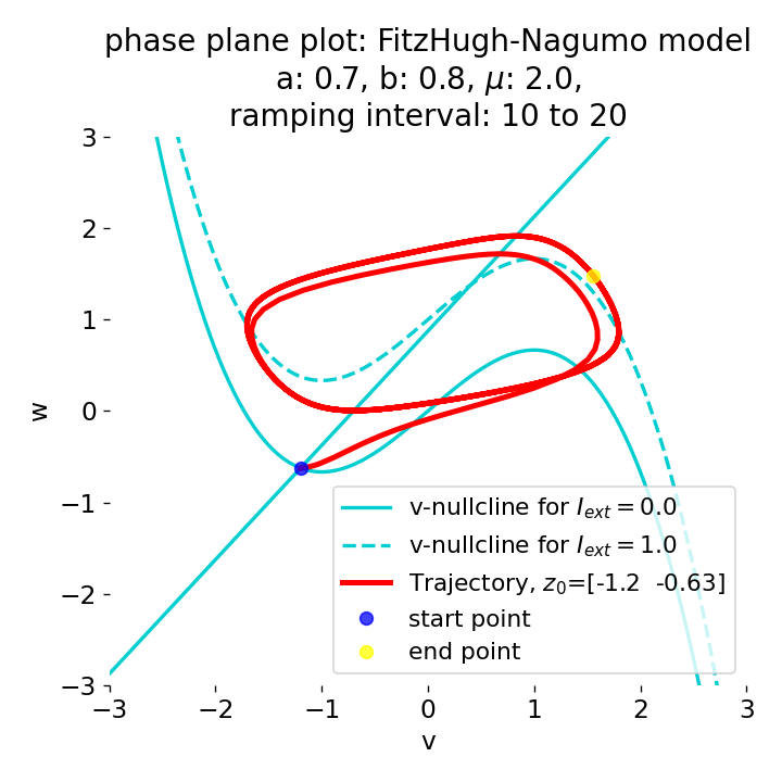
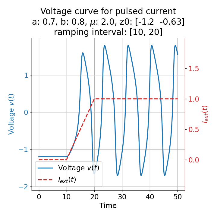
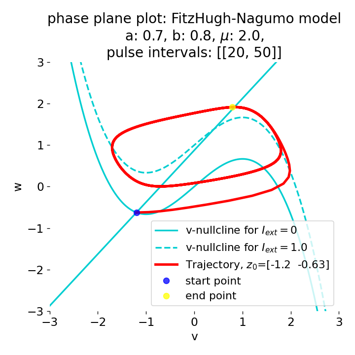
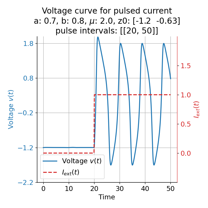Phase plane plots (left) and voltage curves (right) for slowly ramped external current from $I_{\text{ext}}=0.0$ to $I_{\text{ext}}=1.0$ (upper panel) and for an abruptly increased external current from $I_{\text{ext}}=0.0$ to $I_{\text{ext}}=1.0$ (lower panel). In both cases, a spike train is generated. The first action potential of the spike train is a bit higher for the abruptly increased external current, while all action potentials have the same amplitude for the slowly ramped external current (except for the spike(s) that may occur during the ramping period).

Conclusion

The FitzHugh-Nagumo model is a simple two-dimensional system that captures the essential dynamics of neuronal excitability and spike-generating mechanisms. By analyzing the phase plane of the system, we can gain insights into the system’s behavior and understand how different external currents affect the system’s response. The system’s dynamics are highly sensitive to the external input, and small changes in the external current can have a significant impact on the firing behavior of the neuron. The system can exhibit a variety of behaviors, including sub-threshold oscillations, single action potentials, and spike trains, depending on the external current and the system’s initial conditions. The model’s ability to simulate sub-threshold oscillations and stochastic behavior makes it a valuable tool for studying neuronal excitability and spike-generating mechanisms. By applying time-dependent external currents to the system, we can mimic the effect of synaptic inputs on the neuron and study how the neuron responds to different input patterns. The model’s response to different input patterns highlights the critical role of synaptic input timing and frequency in determining neuronal firing behavior.

Overall, the FitzHugh-Nagumo model provides a simple yet powerful framework for studying the dynamics of neuronal excitability and spike generation, and its insights can help us better understand the complex behavior of real neurons. However, we should also bear in mind, that the model is a simplification of the real neuronal dynamics and does not capture all the intricacies of real neurons. For a more detailed and biophysically accurate model, the Hodgkin-Huxley model is often used, which includes additional ion channels and more complex dynamics. Nevertheless, the simplicity of the FitzHugh-Nagumo model makes it a valuable tool for studying the basic principles of neuronal excitability and spike generation and provides a solid foundation for further exploration of more complex models.

You can find the Python code used to generate the plots in this post in this GitHub repositoryꜛ. Feel free to experiment with the code and explore the dynamics of the FitzHugh-Nagumo model further.

References and further reading

• FitzHugh, Impulses and Physiological States in Theoretical Models of Nerve Membrane, 1961, Biophysical Journal, Vol. 1, Issue 6, pages 445-466, doi: 10.1016/s0006-3495(61)86902-6
• FitzHugh R. (1969), Mathematical models of excitation and propagation in nerve. Chapter 1, pp. 1-85 in H.P. Schwan, ed. Biological Engineering, McGraw-Hill Book Co., N.Y., PDF available on ResearchGateꜛ
• FitzHugh, Mathematical models of threshold phenomena in the nerve membrane, 1955, The Bulletin of Mathematical Biophysics, Vol. 17, Issue 4, pages 257-278, doi: 10.1007/BF02477753
• Nagumo, Arimoto, Yoshizawa, An Active Pulse Transmission Line Simulating Nerve Axon, 1962, Proceedings of the IRE, Vol. 50, Issue 10, pages 2061-2070, doi: 10.1109/JRPROC.1962.288235
• Wulfram Gerstner, Werner M. Kistler, Richard Naud, and Liam Paninski, Neuronal Dynamics: From Single Neurons to Networks and Models of Cognition. Chapter 4: Dimensionality Reduction and Phase Plane Analysis, 2014, Cambridge University Press, ISBN: 978-1-107-06083-8
• D. H. Rothman, Lecture notesꜛ for 12.006J/18.353J/2.050J, Nonlinear Dynamics: Bifurcations in two dimensionsꜛ, MIT September 27, 2022
• Ian Cooper, *Doing physics with Python/Matlab: FitzHugh-Nagumo model for spiking neurons*ꜛ
• Scholarpedia article on the FitzHugh-Nagumo modelꜛ