Wasserstein distance via entropy regularization (Sinkhorn algorithm)
In the previous post, we learned about the Wasserstein distance, a metric that quantifies the dissimilarity between two probability distributions. In the field of machine learning, especially in the context of generative models, optimal transport and the Wasserstein distance have become popular tools for comparing probability distributions. However, the computational cost of calculating the Wasserstein distance using methods such as linear programming can be prohibitive, especially for large datasets. This is where alternative calculation methods such as the Sinkhorn algorithm come into play. The Sinkhorn algorithm provides a computationally efficient method for approximating the Wasserstein distance, making it a practical choice for many applications.
Mathematical foundation
Before we head over to the Sinkhorn algorithm, let’s first understand Sinkhorn’s theorem, which is the foundation of the algorithm. The theorem is named after Richard Sinkhorn, who proved it in the context of matrices.
The Sinkhorn theorem states that, given a matrix $A \in \mathbb{R}^{n \times n}$ with positive entries $a_{ij} \gt 0$ for all $i, j$, there exist diagonal matrices $D_1 = \text{diag}(d_1)$ and $D_2 = \text{diag}(d_2)$ with positive diagonal entries such that $D_1 A D_2$ is a doubly stochastic matrix. In other words, all rows and columns of $D_1 A D_2$ sum to one.
The Sinkhorn algorithm, which is used to find these diagonal matrices, can be described as follows:
- Initialize $d_1 = d_2 = \mathbf{1}$ (a vector of ones).
- Repeat until convergence:
- Update $d_1$ by setting $d_1 = \frac{1}{A d_2}$.
- Update $d_2$ by setting $d_2 = \frac{1}{A^T d_1}$.
In the context of optimal transport, the matrix $A$ is typically chosen to be $e^{-C/\epsilon}$, where $C$ is the cost matrix, $\epsilon \gt 0$ is a regularization parameter, and the exponentiation is element-wise. The resulting matrix $P = D_1 A D_2$ is then a near-optimal transport plan, and the value of the regularized optimal transport problem is approximately $\langle P, C \rangle = \text{trace}(P^T C)$.
The Sinkhorn algorithm is efficient because each iteration only involves matrix-vector multiplications and element-wise operations, which can be done in linear time. Furthermore, the algorithm is guaranteed to converge to a unique solution due to the Sinkhorn theorem.
Let’s recap the original optimal transport problem. The goal of the problem is to find a transport plan that minimizes the total cost of transporting mass from one distribution to another:
\[\min_{\gamma \in \Gamma(P, Q)} \langle \gamma, C \rangle\]where $\gamma$ is the transport plan, $C$ is the cost matrix, and $\Gamma(P, Q)$ is the set of all transport plans that move mass from distribution $Q$ to distribution $Q$. The Sinkhorn algorithm addresses this problem by adding an entropy regularization term, which transforms the problem into:
\[\min_{\gamma \in \Gamma(P, Q)} \langle \gamma, C \rangle - \epsilon H(\gamma)\]where $H(\gamma)$ is the entropy of the transport plan, and $\epsilon \gt 0$ is the regularization parameter. The entropy of a transport plan is defined as:
\[H(\gamma) = -\sum_{i,j} \gamma_{i,j} \log(\gamma_{i,j})\]The Sinkhorn algorithm solves this regularized problem by iteratively updating the transport plan according to the following rule:
\[\gamma^{(k+1)} = \text{diag}(u) K \text{diag}(v)\]where $K = \exp(-C/\epsilon)$ is the kernel matrix, $u$ and $v$ are vectors that are updated at each iteration to ensure that the transport plan $\gamma$ satisfies the marginal constraints, and $\text{diag}(u)$ denotes a diagonal matrix with the elements of $u$ on its diagonal.
The Sinkhorn algorithm iterates this update rule until convergence, resulting in a transport plan that minimizes the regularized problem. The resulting transport plan is smoother and less scattered than the one obtained from the original problem, which makes the Sinkhorn algorithm a powerful tool for computing the Wasserstein distance in large-scale problems.
While the Sinkhorn algorithm provides a computationally efficient method for approximating the Wasserstein distance, it’s important to note that the results can differ from those obtained using linear programming. The reason for this is that the Sinkhorn algorithm introduces a regularization term to the optimal transport problem, which can lead to a different solution than the unregularized problem solved by linear programming. When the regularization parameter $\epsilon$ is small, the solution of the Sinkhorn algorithm is close to the solution of the unregularized problem, and the Wasserstein distance calculated with the Sinkhorn algorithm is close to the true Wasserstein distance. However, when $\epsilon$ is large, the solution of the Sinkhorn algorithm can be quite different from the solution of the unregularized problem, and the Wasserstein distance calculated with the Sinkhorn algorithm can be quite different from the true Wasserstein distance. Despite these potential differences in results, the Sinkhorn algorithm remains a practical choice for many applications due to its computational efficiency, especially for large problems.
Python example
Here is a Python code example, that computes the Wasserstein distance between two distributions using the Sinkhorn algorithm. The code is the same we have used in the previous post, except that we exchange the computation of transport plan G. We again use the POT libraryꜛ, which provides an implementation of the Sinkhorn algorithm:
import numpy as np
import matplotlib.pyplot as plt
import ot.plot
from ot.datasets import make_1D_gauss as gauss
from matplotlib import gridspec

# generate the distributions:
n = 100  # nb bins
x = np.arange(n, dtype=np.float64) # bin positions
a = gauss(n, m=20, s=5)  # m= mean, s= std
b = gauss(n, m=60, s=10)

# calculate the cost/loss matrix:
M = ot.dist(x.reshape((n, 1)), x.reshape((n, 1)), metric='sqeuclidean')
M /= M.max()

# solve transport plan problem using Sinkhorn algorithm:
epsilon = 1e-3
G = ot.sinkhorn(a, b, M, epsilon, verbose=False)

# calculate the Wasserstein distance:
w_dist = np.sum(G * M)
print(f"Wasserstein distance W_1: {w_dist}")

# plot distribution:
plt.figure(1, figsize=(6.4, 3))
plt.plot(x, a, c="#0072B2", label='Source distribution', lw=3)
plt.plot(x, b, c="#E69F00", label='Target distribution', lw=3)
ax = plt.gca()
ax.spines['top'].set_visible(False)
ax.spines['right'].set_visible(False)
ax.spines['left'].set_linewidth(2)
ax.spines['bottom'].set_linewidth(2)
ax.tick_params(axis='x', which='major', width=2)
ax.tick_params(axis='y', which='major', width=2)
ax.tick_params(axis='both', which='major', labelsize=12)
plt.legend()
plt.show()

# plot loss matrix:
plt.figure(2, figsize=(5, 5))
plot1D_mat(a, b, M, 'Cost matrix\nC$_{i,j}$')
plt.show()

# plot optimal transport plan:
plt.figure(3, figsize=(5, 5))
plot1D_mat(a, b, G, 'Optimal transport\nmatrix G$_{i,j}$')
plt.show()
The plot function plot1D_mat, which is a modified adaption from the POT library, also remains unchanged:
def plot1D_mat(a, b, M, title=''):
    """ Plot matrix :math:`\mathbf{M}`  with the source and target 1D distribution

    Creates a subplot with the source distribution :math:`\mathbf{a}` on the left and
    target distribution :math:`\mathbf{b}` on the top. The matrix :math:`\mathbf{M}` is shown in between.

    Modified function from the POT library.

    Parameters:
    ----------
    a : ndarray, shape (na,)
        Source distribution
    b : ndarray, shape (nb,)
        Target distribution
    M : ndarray, shape (na, nb)
        Matrix to plot
    """
    na, nb = M.shape
    gs = gridspec.GridSpec(3, 3)
    xa = np.arange(na)
    xb = np.arange(nb)

    ax1 = plt.subplot(gs[0, 1:])
    plt.plot(xb, b, c="#E69F00", label='Target\ndistribution', lw=2)
    ax1.spines['top'].set_visible(False)
    ax1.spines['right'].set_visible(False)
    plt.ylim((0, max(max(a), max(b))))
    # make axis thicker:
    ax1.spines['left'].set_linewidth(1.5)
    ax1.spines['bottom'].set_linewidth(1.5)
    plt.legend(fontsize=8)

    ax2 = plt.subplot(gs[1:, 0])
    plt.plot(a, xa, c="#0072B2",  label='Source\ndistribution', lw=2)
    plt.xlim((0, max(max(a), max(b))))
    plt.xticks(ax1.get_yticks())
    plt.gca().invert_xaxis()
    plt.gca().invert_yaxis()
    ax2.spines['top'].set_visible(False)
    ax2.spines['right'].set_visible(False)
    ax2.spines['left'].set_linewidth(1.5)
    ax2.spines['bottom'].set_linewidth(1.5)
    plt.legend(fontsize=8)

    plt.subplot(gs[1:, 1:], sharex=ax1, sharey=ax2)
    plt.imshow(M, interpolation='nearest', cmap="plasma")
    ax = plt.gca()
    plt.axis('off')
    plt.text(xa[-1:], 0.5, title, horizontalalignment='right', verticalalignment='top',
             color='white', fontsize=12, fontweight="bold")
    plt.xlim((0, nb))
    plt.tight_layout()
    plt.subplots_adjust(wspace=0., hspace=0.2)
Here is how the two distributions look like:
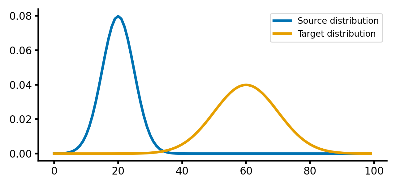 Source and target distributions, $P$ and $Q$, respectively. The Wasserstein distance measures the minimum cost of transporting mass from the source distribution to the target distribution.
The cost matrix:
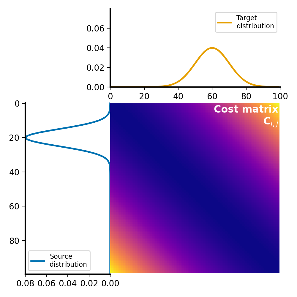 The cost matrix $C$ remains unchanged compared to the calculation of the Wasserstein distance using linear programming. THe Sinkhorn algorithm only approximates the transport plan $G$.
And the resulting transportation plan, compared to the transportation calculated with linear programming:
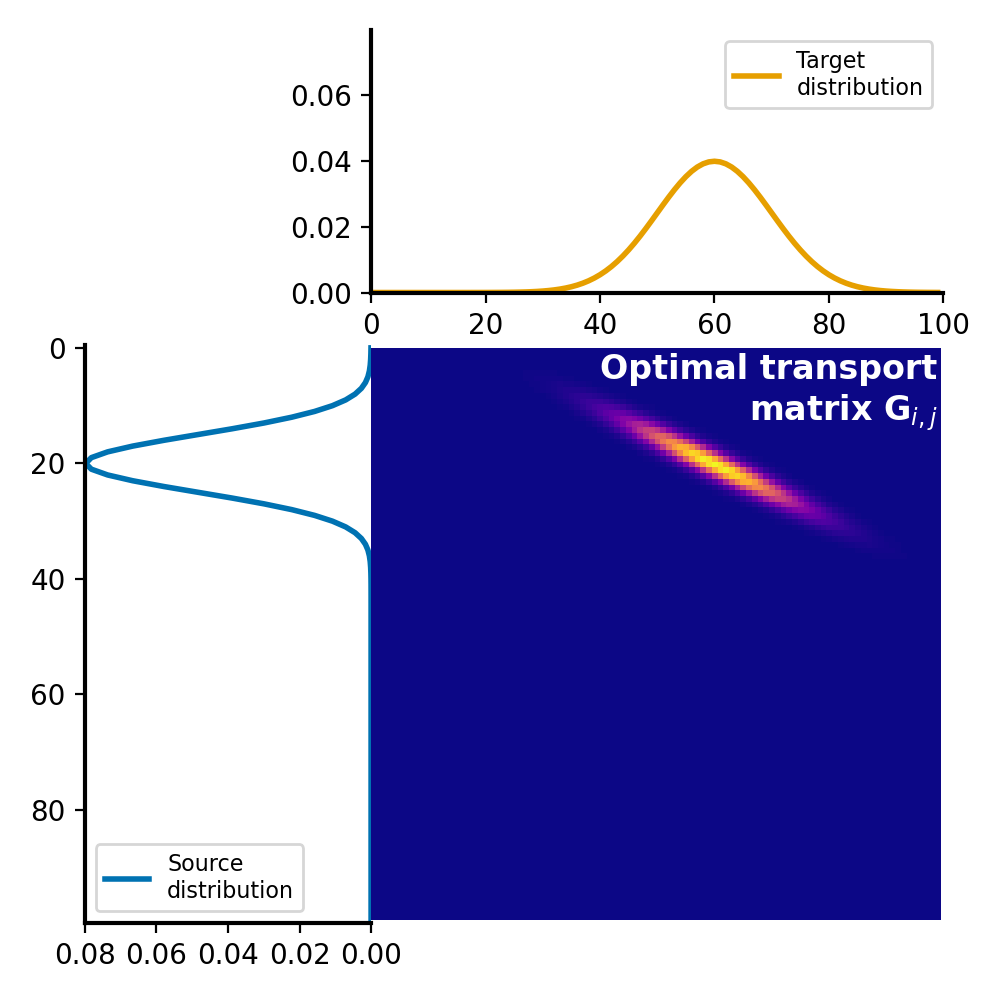 Optimal transport plan $G$ calculated with Sinkhorn algorithm.
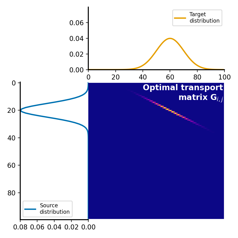 Optimal transport plan $G$ calculated with linear programming.
The corresponding Wasserstein distance is $W_1 = \sim0.1662$ and $W_1 = \sim0.1658$ for the Sinkhorn algorithm and linear programming, respectively. The difference is small, but it’s important to keep in mind that the Sinkhorn algorithm only approximates the optimal transport plan, which can lead to differences in the resulting Wasserstein distance.
Conclusion
The Sinkhorn algorithm offers an efficient solution to the optimal transport problem and the calculation of the Wasserstein distance. By introducing regularization, it makes the problem computationally tractable for large datasets, a task that is often infeasible with traditional linear programming methods. However, the regularization can lead to differences in the results, controlled by the regularization parameter, epsilon. Therefore, a careful balance between computational efficiency and result accuracy is crucial.
The code used in this post is available in this GitHub repositoryꜛ.
If you have any questions or suggestions, feel free to leave a comment below or reach out to me on Mastodonꜛ.
References and further reading
- Cuturi, “Sinkhorn distances: Lightspeed computation of optimal transport.” Advances in neural information processing systems, 2013. arXiv:1306.0895ꜛ
- Chizat et al., “Faster Wasserstein Distance Estimation with the Sinkhorn Divergence”, Neural Information Processing Systems, Dec 2020, Vancouver, Canada, 2020. arXiv:2006.08172ꜛ

Comments
Comment on this post by publicly replying to this Mastodon post using a Mastodon or other ActivityPub/Fediverse account.
Comments on this website are based on a Mastodon-powered comment system. Learn more about it here.
There are no known comments, yet. Be the first to write a reply.