Using random forests for pixel classification

In my previous post I’ve compared random forests to decision trees in both classification and regression tasks. While exploring the classification aspect of random forests, it is worth noting that their applications can be extended beyond traditional classification problems. One such extension is the utilization of random forests for pixel classification, where they prove to be effective. In this post, we will delve into that domain and explore how random forests can be employed to tackle pixel classification tasks.

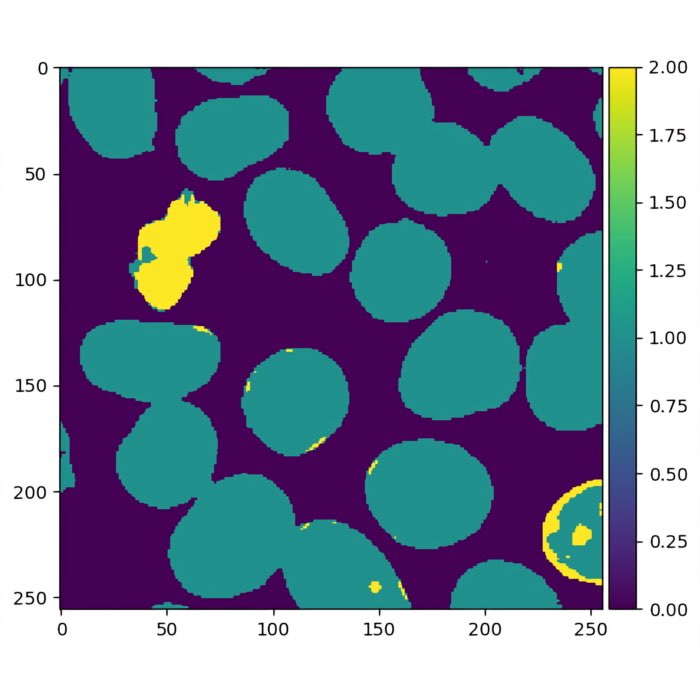
Pixel or image classification involves assigning class labels to individual pixels within an image based on their features. Random forest, as an ensemble learning method, can effectively handle pixel classification problems. Here is a rough overview of how random forest can be used for pixel classification tasks:

• Step 1 – Feature Extraction: The first step in pixel classification is to extract relevant features from the pixels. These features can include pixel intensity, color values, texture information, or other image descriptors. The features are extracted from labeled training images where the class labels for each pixel are known.
• Step 2 – Training Data Preparation: The labeled training images are used to create a training dataset, where each pixel’s features are paired with the corresponding class label. The feature vectors serve as the input features, and the class labels act as the target variable.
• Step 3 – Random Forest Training: The random forest algorithm is trained on the training dataset, where each decision tree in the forest is built using random subsets of the training data and features. The trees are trained to predict the class labels based on the provided features.
• Step 4 – Pixel Classification: Once the random forest model is trained, it can be used to classify the unlabeled pixels in a new image. The features of each pixel in the new image are input to the trained random forest model, which predicts the corresponding class label for that pixel.
• Step 5 – Post-processing: Post-processing techniques like majority voting or filtering can be applied to enhance the classification results and reduce noise or misclassifications.

Random forests are well-suited for pixel classification tasks because they can handle high-dimensional feature spaces, capture complex relationships between features and class labels, and provide robust predictions. They are also less prone to overfitting compared to individual decision trees.

To apply Random Forest for pixel classification, it’s important to carefully select and extract relevant features from the image pixels. Additionally, obtaining a representative and diverse training dataset with accurate class labels is crucial for training an effective model.

It’s worth noting that other machine learning techniques such as deep learning-based convolutional neural networks (CNNs) have gained popularity in pixel classification tasks due to their ability to automatically learn hierarchical features. However, random forests remain a viable option, particularly for scenarios with limited training data or when interpretability is desired.

Practical implementation in Python

Let’s demonstrate the usage of a random forests for pixel classification in Python. I acknowledge, that the following code is based on this tutorialꜛ by Robert Haase.

For reproducibility:

conda create -n random_forest_vs_decision_tree -y python=3.9
conda activate random_forest_vs_decision_tree
conda install -y mamba
mamba install -y scikit-learn matplotlib numpy ipykernel pandas scikit-image napari[all]

Let’s first load a sample image and interactively annotate some parts of it using Napari. The sample image is the z-projection of the nuclei layer of the Cells3D image from the scikit-image sample dataset:

from sklearn.ensemble import RandomForestClassifier
from skimage.io import imread, imshow
import numpy as np
import napari
from skimage import data, filters
import matplotlib.pyplot as plt
# %% LOAD AND ANNOTATE THE IMAGE
# Load the cells3D image:
image = data.cells3d()

# extract the nuclei channel and z-project:
image_2D = image[:, 1, ...].max(axis=0)

# interactively label the nuclei:
# start napari and add image:
viewer = napari.Viewer()
viewer.add_image(image_2D)
# add an empty labels layer:
labels = viewer.add_labels(np.zeros(image_2D.shape).astype(int))

The code above loads and prepares the sample image and opens it in Napari together with a new label layer. Label some of the two different types of nuclei (nucleus type-I and type-II, use label number 2 and 3) and background pixels (label 1) in the label layer. When you’re done, execute the next code part to review your annotations and load the label layer back into the main program execution:

# %% VIEW ANNONTATIONS
# take a screenshot of the annotation:
napari.utils.nbscreenshot(viewer)
# retrieve the annotations from the napari layer:
annotations = labels.data

# plot the original image and the annotations side-by-side in a subplot:
fig, axes = plt.subplots(ncols=2, figsize=(8, 4))
axes[0].imshow(image_2D)
axes[0].set_title('Original image')
axes[1].imshow(annotations)
axes[1].set_title('Annotations')
plt.show()

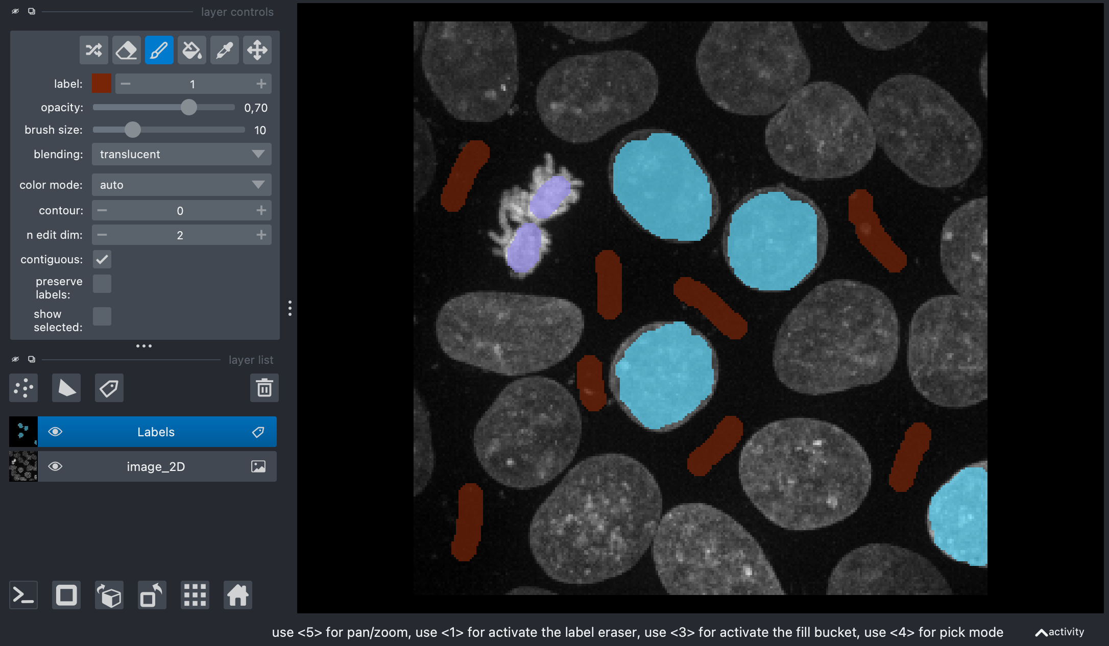Screenshot of Napari showing the original image and my annotations on the label layer.

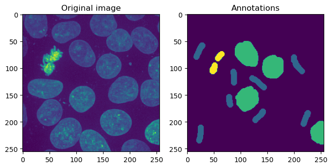The original image side-by-side with the annotations.

The next steps includes the feature extraction of the image. We decided for two extra features:

• the pixel values after applying Gaussian blur (=denoising)
• the pixel values of the Gaussian blurred image processed through a Sobel operator (=edge detection)

Together with the original pixel values we will get a 3D feature stack:

def generate_feature_stack(image):
    # determine features
    blurred = filters.gaussian(image, sigma=2)
    edges = filters.sobel(blurred)

    """
    Collect features in a stack. The ravel() function turns a nD image into 
    a 1-D image. We need to use it because scikit-learn expects values in a 
    1-D format here. 
    """
    feature_stack = [image.ravel(),
                     blurred.ravel(),
                     edges.ravel()]
    
    return np.asarray(feature_stack)

feature_stack = generate_feature_stack(image_2D)

and view the feature stack:

# show feature images:
fig, ax = plt.subplots(1, 3, figsize=(10,10))
# reshape(image.shape) is the opposite of ravel() here. We just need it for visualization.
ax[0].imshow(feature_stack[0].reshape(image_2D.shape), cmap=plt.cm.gray)
ax[0].set_title('Original image')
ax[1].imshow(feature_stack[1].reshape(image_2D.shape), cmap=plt.cm.gray)
ax[1].set_title('Blurred image')
ax[2].imshow(feature_stack[2].reshape(image_2D.shape), cmap=plt.cm.gray)
ax[2].set_title('Edges')
plt.show()

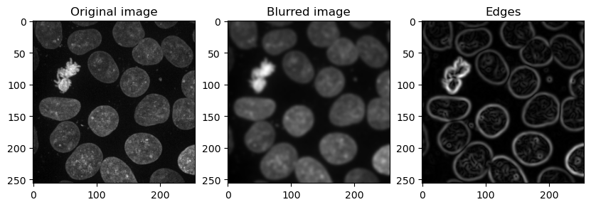The feature stack consisting of the layer with the original pixel values, the pixel values after applying Gaussian blur (=denoising), and the pixel values of the Gaussian blurred image processed through a Sobel operator (=edge detection).

Next, we need to format the input data so that it fits to what scikit-learn expects. scikit-learn expects an array of shape $(n, m)$ as input data and $n$ annotations, where $n$ corresponds to the number of pixels and $m$ to number of features (in our case $m = 3$):

# %% FORMATTING DATA
def format_data(feature_stack, annotation):
    # reformat the data to match what scikit-learn expects
    # transpose the feature stack
    X = feature_stack.T
    # make the annotation 1-dimensional
    y = annotation.ravel()
    
    # remove all pixels from the feature and annotations which have not been annotated
    mask = y > 0
    X = X[mask]
    y = y[mask]

    return X, y

X, y = format_data(feature_stack, annotations)

print("input shape", X.shape)
print("annotation shape", y.shape)

input shape (8795, 3)
annotation shape (8795,)

Now, we can train the random forest and predict the classes for the unlabeled pixels:

# %% TRAIN AND PREDICT WITH RANDOM FOREST CLASSIFIER
classifier = RandomForestClassifier(max_depth=10, random_state=0)
classifier.fit(X, y)
RandomForestClassifier(max_depth=2, random_state=0)

result = classifier.predict(feature_stack.T) - 1 # we subtract 1 to make background = 0
result_2d = result.reshape(image_2D.shape)
imshow(result.reshape(image_2D.shape))
viewer.add_labels(result_2d)
napari.utils.nbscreenshot(viewer)

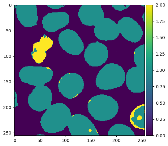Predictions by the trained random forest classifier.

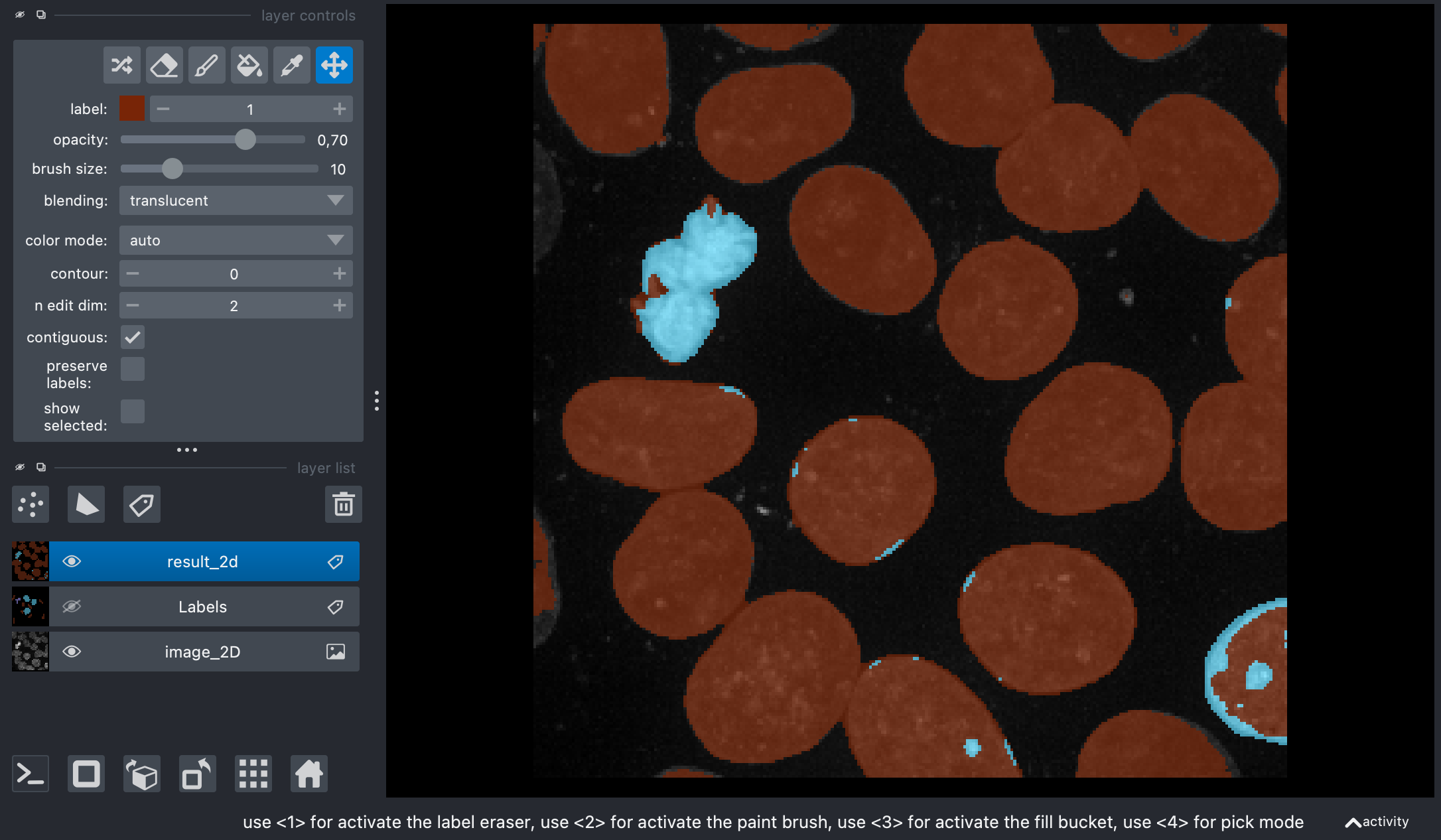Predictions by the trained random forest classifier overlayed on the original image in Napari.

The two plots above are our final result. The random forest classifier demonstrates its capability to classify pixels belonging to the two nuclei types as well as pixels representing the background. However, the classifier is not perfect and there are still some misclassifications, particularly in identifying bright type-I nuclei as type-II nuclei. To further improve the classifier, additional annotations or labels can be provided. By incorporating more accurately labeled data during the training process, the random forest model can learn from a larger and more diverse set of examples, potentially leading to enhanced accuracy and reduced misclassifications. Moreover, other strategies such as feature engineering/extraction or adjusting hyperparameters can also contribute to improving the classifier’s performance. By carefully selecting and engineering relevant features, or fine-tuning the model’s parameters, we can aim for better accuracy and more reliable results.

Practical implementation in Python: Another example

Just out of curiosity, let’s apply the random forest to another sample image. This time, we will use the skin image from the same sample dataset:

image_2d_2 = data.skin()[:,:,0]
viewer = napari.Viewer()
viewer.add_image(image_2d_2)
# add an empty labels layer:
labels = viewer.add_labels(np.zeros(image_2d_2.shape).astype(int))

Add some annotations:

# %% SECOND EXAMPLE (SKIN): VIEW ANNONTATIONS
# take a screenshot of the annotation:
napari.utils.nbscreenshot(viewer)
# retrieve the annotations from the napari layer:
annotations = labels.data

# plot the original image and the annotations side-by-side in a subplot:
fig, axes = plt.subplots(ncols=2, figsize=(8, 4))
axes[0].imshow(image_2d_2)
axes[0].set_title('Original image')
axes[1].imshow(annotations)
axes[1].set_title('Annotations')
plt.show()

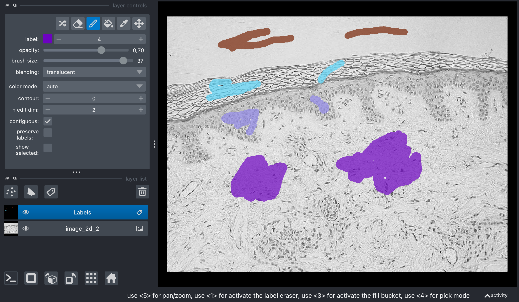Screenshot of Napari showing the original image and my annotations on the label layer.

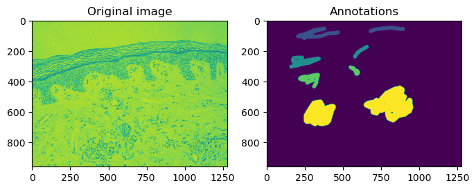The original image side-by-side with the annotations.

Generate the image feature stack:

# %% GENERATE IMAGE FEATURE STACK
feature_stack = generate_feature_stack(image_2d_2)

# show feature images:
fig, ax = plt.subplots(1, 3, figsize=(10,10))
# reshape(image.shape) is the opposite of ravel() here. We just need it for visualization.
ax[0].imshow(feature_stack[0].reshape(image_2d_2.shape), cmap=plt.cm.gray)
ax[0].set_title('Original image')
ax[1].imshow(feature_stack[1].reshape(image_2d_2.shape), cmap=plt.cm.gray)
ax[1].set_title('Blurred image')
ax[2].imshow(feature_stack[2].reshape(image_2d_2.shape), cmap=plt.cm.gray)
ax[2].set_title('Edges')
plt.show()

The feature stack consisting of the layer with the original pixel values, the pixel values after applying Gaussian blur (=denoising), and the pixel values of the Gaussian blurred image processed through a Sobel operator (=edge detection).

Format the data:

X, y = format_data(feature_stack, annotations)
print("input shape", X.shape)
print("annotation shape", y.shape)

input shape (112990, 3)
annotation shape (112990,)

And train the classifier and predict the classes of the unlabeled pixels:

# %% TRAIN AND PREDICT WITH RANDOM FOREST CLASSIFIER
classifier = RandomForestClassifier(max_depth=10, random_state=0, max_samples=0.05, n_estimators=50)
classifier.fit(X, y)
RandomForestClassifier(max_depth=2, random_state=0)

result = classifier.predict(feature_stack.T) - 1 # we subtract 1 to make background = 0
result_2d = result.reshape(image_2d_2.shape)
imshow(result.reshape(image_2d_2.shape))
viewer.add_labels(result_2d)
napari.utils.nbscreenshot(viewer)

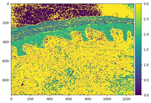Predictions by the trained random forest classifier.

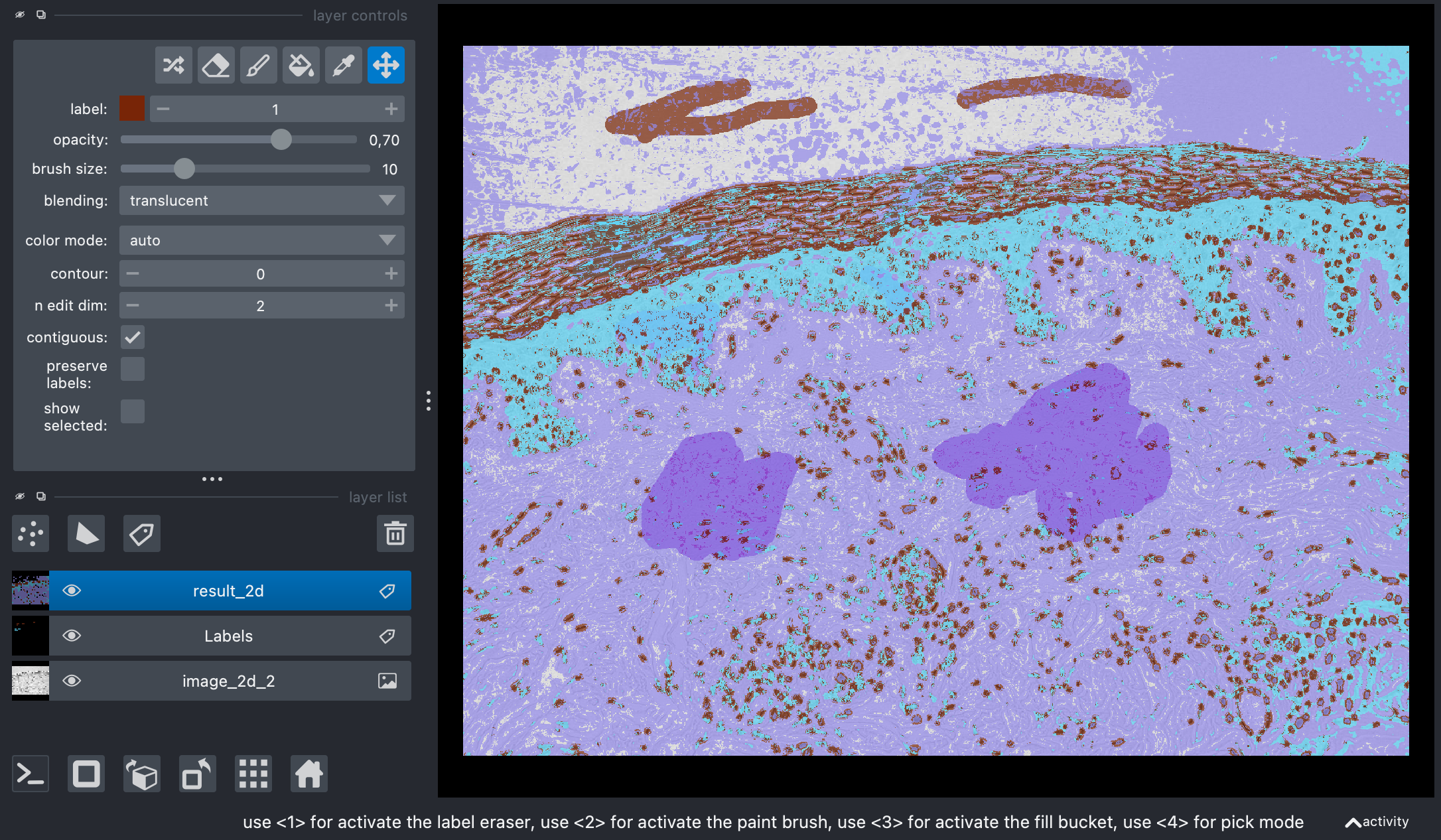Predictions by the trained random forest classifier overlayed on the original image and the label layer in Napari.

Again, the classifier is able to identify the different tissue types in the sample image. However, it has difficulties to perform the classification accurately. The same measures to improve the accuracy mentioned above account here as well.

Conclusion

Random forests have demonstrated their effectiveness in pixel classification, where class labels are assigned to individual pixels within an image based on their features. By following the outlined steps, including feature extraction, training data preparation, random forest training, pixel classification, and post-processing, random forests can be successfully applied to tackle pixel classification tasks. Despite the rise of deep learning techniques like Convolutional Neural Networks (CNN), random forests remain a valuable option, especially in scenarios with limited training data or when interpretability is desired. Careful feature selection and obtaining a diverse and accurate training dataset are crucial for training an effective random forest model.

The code for this post can be found in this GitHub repositoryꜛ

And as usual, if you have any questions or suggestions, feel free to leave a comment below or reach out to me on Mastodonꜛ.