Understanding gradient descent in machine learning
Gradient descent is a fundamental optimization algorithm widely used in machine learning for finding the optimal parameters of a model. It is a powerful technique that enables models to learn from data by iteratively adjusting their parameters to minimize a cost or loss function. In this blog post, we explore the mathematical background of this method and showcase its implementation in Python.
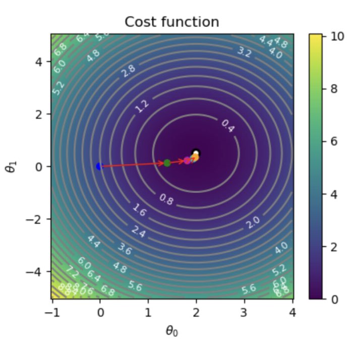
The mathematics behind gradient descent
Gradient descent is an optimization algorithm used to minimize the cost function of a machine learning model. Its main idea revolves around iteratively adjusting the model’s parameters in the direction of the steepest descent of the cost function, aiming to reach the global or local minimum.
The mathematical formulation of gradient descent can be represented as follows:
The goal is to fit a so-called hypothesis function $h_\theta(x)$ to a given dataset $(x^{(i)}, y^{(i)})$ (with $i=1, 2,\ldots, m$) by minimizing the cost function $J(\theta)$ in terms of the parameters $\theta_j$ (with $j=0, 1, \ldots$). $h_\theta(x)$ is defined according to the model we want to use.
Given a cost function $J(\theta)$, where $\theta$ represents the model’s parameters, we aim to find the values of $\theta$ that minimize $J(\theta)$. A common definition of $J(\theta)$ is the mean squared error (MSE) between the predicted values and the actual data, divided by 2,
\[J(\theta) = \frac{1}{2m} \sum_i^m (h_\theta(x^{(i)} - y^{(i)} ))^2.\]Starting with an initial guess for $\theta$, the gradient descent algorithm iteratively updates $\theta$ using the following update rule:
\[\theta_{j} := \theta_{j} - \alpha \frac{\partial J(\theta)}{\partial \theta_{j}}\]Here, $\alpha$ denotes the learning rate, which controls the step size of each iteration. The learning rate determines how quickly the algorithm converges to the optimal solution, with smaller values leading to slower convergence but potentially more precise results.
Python code example for fitting one parameter
Now, let’s demonstrate the implementation of gradient descent using Python code. We will need nothing more than the NumPy and Matplotlib libraries for this purpose. The main code is based on the blog post “Visualizing the gradient descent method”ꜛ from scipython.comꜛ.
We define the hypothesis function (hypothesis function) as a straight line,
plotted on the left panel of the figure below. Thus, our problem is 1D and we only fit one parameter $\theta_1$. The data points are generated from the line $y = 0.5 x$. The cost function $J(\theta_1)$ (cost_func(theta1)) is plotted on the right panel. It visualized how closely the current estimate of $\theta$ is to the optimal solution, i.e., the minimum. The cost function is minimized when the predicted values are equal to the actual data, i.e., when the line fits the data perfectly (left panel).
The following code is implemented in an interactive Jupyter notebook and you can change the main parameters of the algorithm using sliders:
- the step size $N$
- the learning rate $\alpha$
- the initial parameter value $\theta_1$
You can run the notebook in Google Colab or Binder by clicking on one of the buttons below:
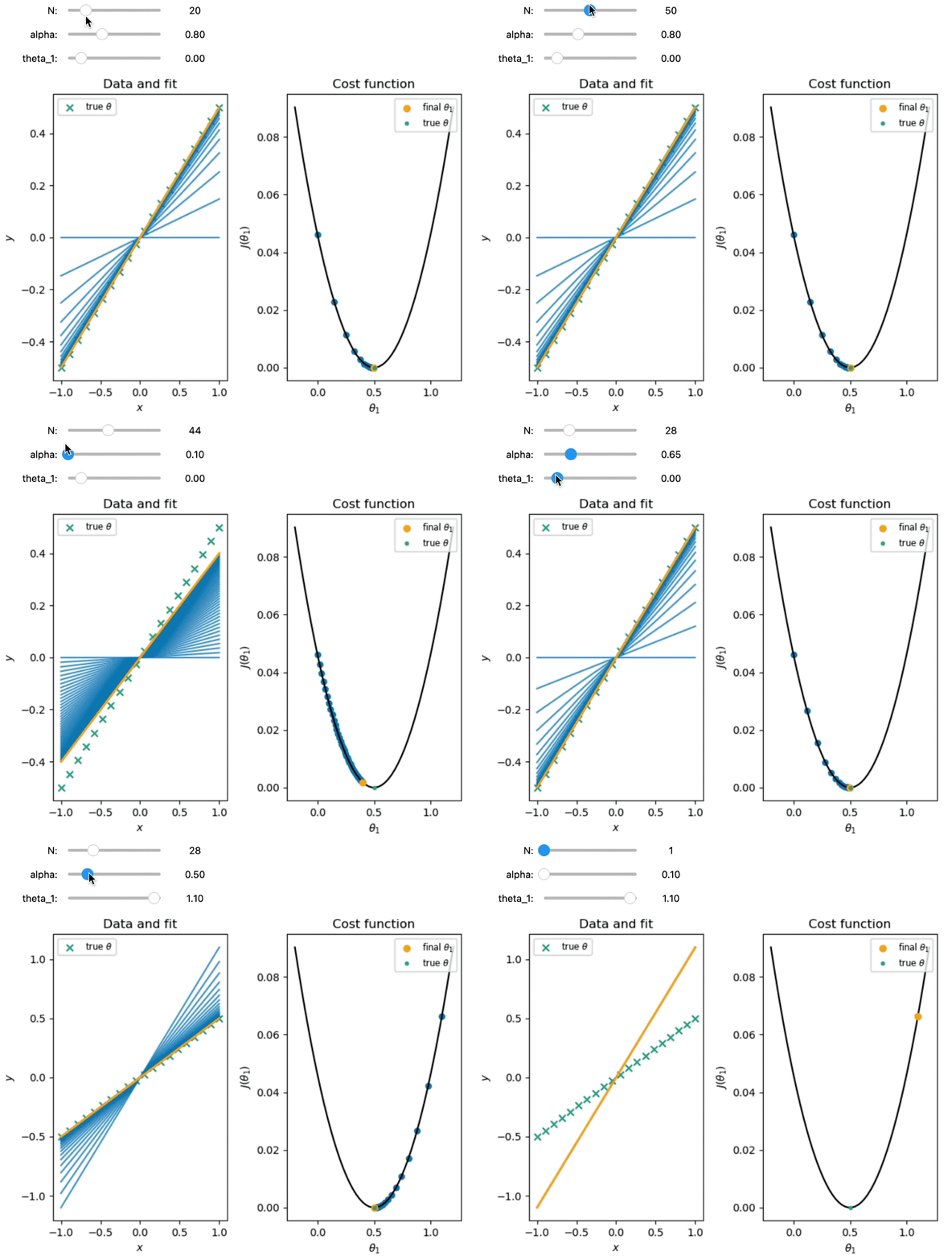 Demonstration of gradient descent for fitting one parameter. The left panel shows the data and the fit for each iteration of the algorithm. The right panel shows the cost function as a function of the parameter $\theta_{1}$ and the steps taken by the algorithm to minimize the cost function. The orange dot indicates the final value of $\theta_{1}$ obtained by the algorithm. The blue dots indicate the values of $\theta_{1}$ at each iteration of the algorithm. The red arrows indicate the steps taken by the algorithm to minimize the cost function. The green dot indicates the true value of $\theta_{1}$.
For reproducibility:
conda create -n gradient_descent -y python=3.9
conda activate gradient_descent
conda install -y mamba
mamba install -y ipykernel numpy matplotlib ipywidgets notebook
Here is the code:
import numpy as np
import matplotlib.pyplot as plt
import ipywidgets as widgets
from IPython.display import display

# define the main parameters of the algorithm:
theta1_true = 0.5
m = 20
x = np.linspace(-1, 1, m)
y = theta1_true * x

def update_plot(N, alpha, theta1):
    # Clear previous plot
    plt.clf()

    def cost_func(theta1):
        """The cost function, J(theta1) describing the goodness of fit."""
        theta1 = np.atleast_2d(np.asarray(theta1))
        return np.average((y - hypothesis(x, theta1))**2, axis=1) / 2

    def hypothesis(x, theta1):
        """Our "hypothesis function", a straight line through the origin."""
        return theta1 * x

    # First construct a grid of theta1 parameter pairs and their corresponding
    # cost function values.
    theta1_grid = np.linspace(-0.2, 1.2, 50)
    J_grid = cost_func(theta1_grid[:, np.newaxis])

    # The cost function as a function of its single parameter, theta1.
    plt.subplot(121)
    plt.scatter(x, y, marker='x', s=40, color='#009E73', label=r"true $\theta$")
    plt.xlabel(r'$x$')
    plt.ylabel(r'$y$')
    plt.title('Data and fit')

    # Take N steps with learning rate alpha down the steepest gradient,
    # starting at theta1.
    theta1_values = [theta1]
    J_values = [np.array(cost_func(theta1_values[0])[0])]
    for j in range(N - 1):
        last_theta1 = theta1_values[-1]
        this_theta1 = last_theta1 - alpha / m * np.sum(
            (hypothesis(x, last_theta1) - y) * x)
        theta1_values.append(this_theta1)
        J_values.append(np.array(cost_func(this_theta1)[0]))

    # Annotate the cost function plot with coloured points indicating the
    # parameters chosen and red arrows indicating the steps down the gradient.
    # Also plot the fit function on the LHS data plot.
    for j in range(N):
        plt.plot(x, hypothesis(x, theta1_values[j]), lw=1.5, c="#0072B2", alpha=0.75)
    plt.plot(x, hypothesis(x, theta1_values[j]), lw=2, c="orange")
    plt.legend(loc='upper left', fontsize='small')

    plt.subplot(122)
    plt.plot(theta1_grid, J_grid, 'k')
    plt.scatter(theta1_values, J_values, s=40, lw=0, c="#0072B2")
    plt.plot(theta1_values[-1:], J_values[-1:], 'o', c="orange", label=r"final $\theta_1$")
    plt.plot(theta1_true, 0, '.', c="#009E73", label=r"true $\theta$")
    #plt.xlim(-0.2, 1.2)
    plt.legend(loc='upper right', fontsize='small')
    plt.xlabel(r'$\theta_1$')
    plt.ylabel(r'$J(\theta_1)$')
    plt.title('Cost function')

    plt.tight_layout()
    plt.show()

# Create sliders
slider_N = widgets.IntSlider(value=20, min=1, max=100, description='N:')
slider_alpha = widgets.FloatSlider(value=1.15, min=0.1, max=2.0, step=0.05, description='alpha:')
slider_theta1 = widgets.FloatSlider(value=0.0, min=-0.2, max=1.2, step=0.05, description='theta_1:')

# Register the update_plot function as the callback for each slider using interactive
interactive_plot = widgets.interactive(update_plot, N=slider_N, alpha=slider_alpha, theta1=slider_theta1)

# Display the interactive plot
display(interactive_plot)
$\theta_{1, \text{true}}$ (theta1_true) represents the true or ideal value of the parameter $\theta_{1}$ that we are trying to estimate using the gradient descent algorithm. The goal is to find the optimal value of the parameter $\theta_{1}$ that minimizes the cost function, which measures the goodness of fit between the predicted values and the actual data. By iteratively updating the $\theta_{1}$ value based on the gradient of the cost function, the algorithm attempts to converge to the true or ideal value of theta1 that produces the best fit to the data. In our case, $\theta_{1, \text{true}}$ is set to 0.5 as an example. By comparing the estimated $\theta_{1}$ values obtained from the gradient descent algorithm to the true value, we can assess the accuracy and effectiveness of the algorithm in finding the optimal parameter value.
Python code example for fitting two parameters
Now we extend the problem by defining a hypothesis function with two parameters,
\[h_\theta(x) = \theta_0 + \theta_1 x.\]This time, we visualize $J(\theta_0,\theta_1)$ as a contour plot (right panel). The rest follows the same procedure as described above.
The following code is also implemented in an interactive Jupyter notebook and you can change the main parameters of the algorithm using sliders:
- the step size $N$
- the learning rate $\alpha$
- the true parameter value $\theta_0$ and $\theta_1$
- the initial parameter value $\theta_0$ and $\theta_1$
You can run the notebook in Google Colab or Binder by clicking on one of the buttons below:
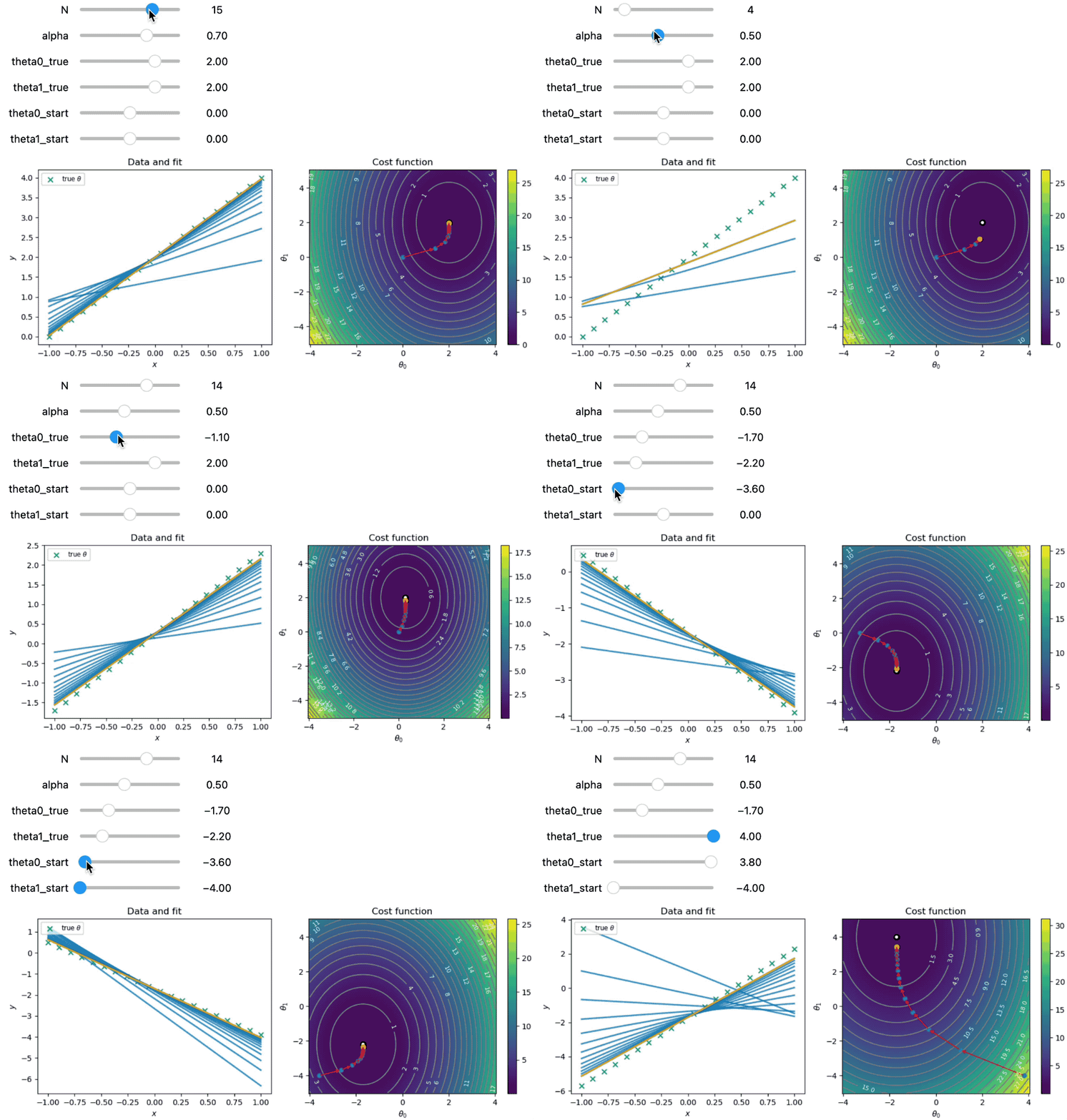 Demonstration of gradient descent for two parameters. The left panel shows the data and the fit function at each iteration. The right panel shows the cost function and the path taken by gradient descent. The orange dot indicates the final parameter values. The red arrows indicate the steps taken by gradient descent. The blue dots indicate the parameter values at each iteration. The white contour lines indicate the parameter values chosen by gradient descent.
Here is the code:
import numpy as np
import matplotlib.pyplot as plt
from ipywidgets import interact, FloatSlider, IntSlider

# The data to fit
m = 20
x = np.linspace(-1, 1, m)
y = None

def cost_func(x, y, theta0, theta1):
    """The cost function, J(theta0, theta1) describing the goodness of fit."""
    return np.average((y - hypothesis(x, theta0, theta1.reshape(-1, 1))) ** 2, axis=1) / 2

def hypothesis(x, theta0, theta1):
    """Our "hypothesis function", a straight line."""
    return theta0.reshape(-1, 1) + theta1 * x

def update_plots(N, alpha, theta0_true, theta1_true, theta0_start, theta1_start):
    global y

    # Generate new y values based on the updated true theta values
    y = theta0_true + theta1_true * x

    # Create the figure and axes objects
    fig, ax = plt.subplots(nrows=1, ncols=2, figsize=(10, 4.15))

    # Initialize the scatter plot for data points
    ax[0].scatter(x, y, marker='x', s=40, color='#009E73', label=r"true $\theta$")

    # Take N steps with learning rate alpha down the steepest gradient,
    # starting at (theta0, theta1) = (theta0_start, theta1_start).
    theta = [np.array((theta0_start, theta1_start))]
    J = [cost_func(x, y, *theta[0])]
    for j in range(N - 1):
        last_theta = theta[-1]
        this_theta = np.empty((2,))
        this_theta[0] = last_theta[0] - alpha / m * np.sum(
            (hypothesis(x, *last_theta) - y))
        this_theta[1] = last_theta[1] - alpha / m * np.sum(
            (hypothesis(x, *last_theta) - y) * x)
        theta.append(this_theta)
        J.append(cost_func(x, y, *this_theta))

    # First construct a grid of (theta0, theta1) parameter pairs and their
    # corresponding cost function values.
    theta0_grid = np.linspace(-4, 4, 101)
    theta1_grid = np.linspace(-5, 5, 101)
    X, Y = np.meshgrid(theta0_grid, theta1_grid)
    J_grid = cost_func(x, y, X.flatten(), Y.flatten()).reshape(X.shape)

    # A pcolor plot for the RHS cost function
    pcolor_plot = ax[1].pcolormesh(X, Y, J_grid, cmap='viridis')
    fig.colorbar(pcolor_plot, ax=ax[1])

    # Contour lines on the pcolor plot
    contours = ax[1].contour(X, Y, J_grid, 30, colors='gray')
    ax[1].clabel(contours, inline=True, fontsize=8, colors='w')

    # The target parameter values indicated on the cost function pcolor plot
    ax[1].scatter([theta0_true] * 2, [theta1_true] * 2, s=[50, 10], color=['k', 'w'])

    # Annotate the cost function plot with coloured points indicating the
    # parameters chosen and red arrows indicating the steps down the gradient.
    # Also plot the fit function on the LHS data plot.
    for j in range(1, N):
        ax[1].annotate('', xy=theta[j], xytext=theta[j - 1],
                       arrowprops={'arrowstyle': '->', 'color': 'r', 'lw': 1},
                       va='center', ha='center')
        ax[0].plot(x, hypothesis(x, *theta[j]).flatten(), lw=2, c="#0072B2", alpha=0.75)
    ax[0].plot(x, hypothesis(x, *theta[j]).flatten(), lw=2, c="#E69F00")
    ax[1].scatter(*zip(*theta), s=40, lw=0)
    last_theta = theta[j]
    ax[1].plot(last_theta[0], last_theta[1], 'o', c="orange")

    # Labels, titles, and a legend.
    ax[1].set_xlabel(r'$\theta_0$')
    ax[1].set_ylabel(r'$\theta_1$')
    ax[1].set_title('Cost function')
    ax[0].set_xlabel(r'$x$')
    ax[0].set_ylabel(r'$y$')
    ax[0].set_title('Data and fit')
    ax[0].legend(loc='upper left', fontsize='small')

    plt.tight_layout()
    plt.show()

# Create sliders
N_slider = IntSlider(min=2, max=20, step=1, value=15)
alpha_slider = FloatSlider(min=0.1, max=1.0, step=0.1, value=0.7)
theta0_true_slider = FloatSlider(min=-4, max=4, step=0.1, value=2)
theta1_true_slider = FloatSlider(min=-4, max=4, step=0.1, value=2)
theta0_start_slider = FloatSlider(min=-4, max=4, step=0.1, value=0)
theta1_start_slider = FloatSlider(min=-4, max=4, step=0.1, value=0)

# Create the interactive widget
interact(update_plots,
         N=N_slider,
         alpha=alpha_slider,
         theta0_true=theta0_true_slider,
         theta1_true=theta1_true_slider,
         theta0_start=theta0_start_slider,
         theta1_start=theta1_start_slider)
Conclusion
Gradient descent is a crucial optimization algorithm widely used in machine learning. By iteratively updating model parameters in the direction of the steepest descent of the cost function, gradient descent enables the optimization of complex models and enhances their predictive power. Understanding and implementing gradient descent empowers machine learning practitioners to fine-tune their models for improved accuracy and efficiency.
Remember to adjust the learning rate and the number of iterations according to your specific problem to achieve the desired results. Happy optimizing!
The entire code used in this post is available in this GitHub repositoryꜛ.
If you have any questions or suggestions, feel free to leave a comment below or reach out to me on Mastodonꜛ.
Comments
Comment on this post by publicly replying to this Mastodon post using a Mastodon or other ActivityPub/Fediverse account.
Comments on this website are based on a Mastodon-powered comment system. Learn more about it here.
There are no known comments, yet. Be the first to write a reply.