The SIR model: A mathematical approach to epidemic dynamics
In the wake of the COVID-19 pandemic, epidemiological models have garnered significant attention for their ability to provide insights into the spread and control of infectious diseases. One such model is the SIR model, an acronym that stands for Susceptible-Infectious-Recovered. Developed by Kermack and McKendrick in the early 20th century, this model forms the foundation for studying the dynamics of epidemics. In this blog post, we delve into the details of the SIR model, providing a mathematical description, and showcasing its application through a Python simulation.
The SIR model
The SIR model divides the population into three distinct compartments: Susceptible ($S$), Infectious ($I$), and Recovered ($R$). The model assumes that the population size remains constant throughout the epidemic and that there is no birth, death, or migration. The primary driving force behind the model is the transmission of the disease from infectious individuals to susceptible ones.
To mathematically describe the SIR model, we use a system of ordinary differential equations (ODEs). Let’s denote the population size as $N$, and the number of individuals in each compartment at time t as $S(t)$, $I(t)$, and $R(t)$, respectively. The flow of individuals between compartments can be described as follows:
1. Susceptible to Infectious ($S\rightarrow I$)
The rate at which susceptible individuals become infected is directly proportional to the number of interactions between susceptible and infectious individuals. This can be expressed as:
\[\frac{dS}{dt} = -\frac{\beta \cdot S \cdot I}{N}\]where $\beta$ represents the contact rate, determining the probability of disease transmission per contact.
2. Infectious to Recovered ($i\rightarrow R$)
The rate at which infectious individuals recover and become immune can be defined as:
\[\frac{dI}{dt} = \frac{\beta \cdot S \cdot I}{N} - \gamma \cdot I\]Here, $\gamma$ represents the mean recovery rate, indicating the average time an individual remains infectious.
3. Recovered individuals ($R$)
The number of individuals transitioning from the infectious compartment to the recovered compartment can be given by:
\[\frac{dR}{dt} = \gamma \cdot I\]It’s important to note that the sum of individuals in all compartments remains constant, as stated by the equation:
\[S + I + R = N\]Python Simulation
To illustrate the application of the SIR model, we will simulate its behavior using Python. For a more meaningful demonstration, we will fit the model to a real example dataset from a influenza outbreak in a British boarding school published in a 1978 issue of the British Medical Journalꜛ. I acknowledge that the main code is based on this blog postꜛ and this documentation pageꜛ. I have made some modifications to the code to make it more readable and understandable.
The Python libraries NumPy, Matplotlib and Scipy are everything what we need to implement the SIR model equations and fit the model to the provided dataset. By adjusting the values of $beta$ and $gamma$ (in 1/days) during the fitting process, we can determine the best estimates that match the observed data.
For reproducibility:
conda create -n sir_model_covid19 -y python=3.9
conda activate sir_model_covid19
conda install -y mamba
mamba install -y pandas matplotlib numpy scipy scikit-learn ipykernel notebook ipympl mplcursors
Let’s prepare the simulation by setting up some initial values:
import matplotlib.pyplot as plt
from scipy.optimize import minimize
import numpy as np
from scipy.integrate import odeint

# set total population:
N = 1000
# define initial number of infected and recovered individuals, I0 and R0:
I0, R0 = 1, 0
# everyone else is susceptible to infection initially, S0:
S0 = N - I0 - R0
# define contact rate beta and mean recovery rate gamma (in 1/days):
beta, gamma = 0.4, 1./10
# Set a grid of time points (in days):
t = np.linspace(0, 90, 90)  # 90 = 6*15
# create some toy-data. Here: influenza in a British boarding school from 1978.
data = [1, 3, 6, 25, 73, 222, 294, 258, 237, 191, 125, 69, 27, 11, 4]
Next, we define the SIR model differential equations:
# the SIR model differential equations:
def deriv(y, t, N, beta, gamma):
    S, I, R = y
    dSdt = -beta * S * I / N
    dIdt = beta * S * I / N - gamma * I
    dRdt = gamma * I
    return dSdt, dIdt, dRdt
Now, we can simulate the model using the odeint function and the initial conditions defined above:
# set initial conditions vector:
y0 = S0, I0, R0
# integrate the SIR equations over the time grid  t:
ret = odeint(deriv, y0, t, args=(N, beta, gamma))
S, I, R = ret.T
Let’s plot the results:
# plot the data on three separate curves for S(t), I(t) and R(t):
scale_Factor =1

fig = plt.figure(2, facecolor='w')
plt.clf()
ax = fig.add_subplot(111, axisbelow=True)
ax.plot(t, S/scale_Factor,  alpha=0.5, lw=2, label='Susceptible')
ax.plot(t, I/scale_Factor,  alpha=0.5, lw=2, label='Infected')
ax.plot(t, R/scale_Factor,  alpha=0.5, lw=2, label='Recovered with immunity')
ax.plot(np.arange(0,6*15,6),data,"k*:", label='Original Data')

ax.set_xlabel('Time /days')
ax.set_ylabel('Number (1000s)')
ax.yaxis.set_tick_params(length=0)
ax.xaxis.set_tick_params(length=0)
legend = ax.legend()
legend.get_frame().set_alpha(0.5)
for spine in ('top', 'right', 'bottom', 'left'):
    ax.spines[spine].set_visible(False)
plt.title('SIR Model without fit to the data (initial conditions)')
plt.savefig('Model without fit.png', dpi=200)
plt.show()
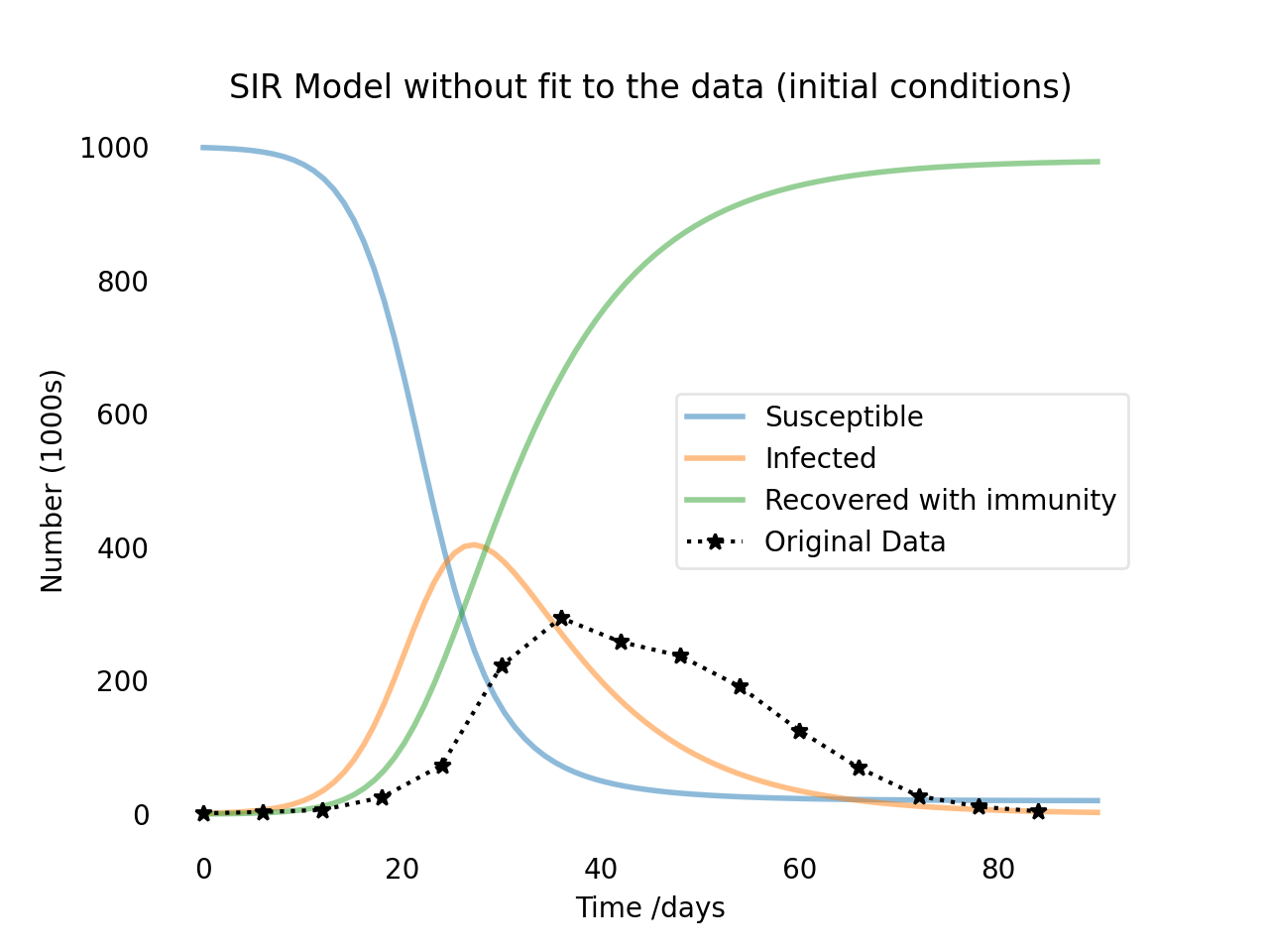 The SIR model without fit to the data (black stars). The shown result serves as a verification of the initial conditions for the subsequent fitting process.
Now that we have a working model, we can fit it to the data. To do this, we need to define a function that calculates the sum of squared errors between the model and the data:
# define the sum of squares function:
def sumsq(p, data, t, N):
    beta, gamma = p
    ret = odeint(deriv, y0, t, args=(N, beta, gamma))
    sum_stepSize = int(len(ret[:,1])/len(data))
    return(sum((ret[::sum_stepSize, 1]-data)**2))
With this function, we can now use the minimize function to find the optimal parameters that minimize the sum of squared errors:
# set initial conditions vector:
p=[0.001,1]
# minimize the sum of squares function
msol = minimize(sumsq, p, (data, t, N), method='Nelder-Mead')

beta_fit, gamma_fit = msol.x

# integrate the SIR equations over the time grid t:
ret_fit = odeint(deriv, y0, t, args=(N, beta_fit, gamma_fit))
S_fit, I_fit, R_fit = ret_fit.T
Let’s plot the results:
# plot the data on three separate curves for S(t), I(t) and R(t):
scale_Factor =1

fig = plt.figure(3, facecolor='w')
plt.clf()
ax = fig.add_subplot(111, axisbelow=True)
ax.plot(t, S_fit/scale_Factor,  alpha=0.5, lw=2, label='Susceptible')
ax.plot(t, I_fit/scale_Factor,  alpha=0.5, lw=2, label='Infected (modelled)')
ax.plot(t, R_fit/scale_Factor,  alpha=0.5, lw=2, label='Recovered with immunity')
ax.plot(np.arange(0,6*15,6),data,"k*:", label='Original Data')

ax.set_xlabel('Time /days')
ax.set_ylabel('Number (1000s)')
# ax.set_ylim(0,1.2)
ax.yaxis.set_tick_params(length=0)
ax.xaxis.set_tick_params(length=0)
legend = ax.legend()
legend.get_frame().set_alpha(0.5)
ax.text(5, 600,
        (r'$\beta_{model} =$' f'{beta_fit.round(2)}\n'
         r'$\gamma_{model} =$' f'{gamma_fit.round(2)}\n\n'
         r'$\Rightarrow \; R_0 =$' f'{(beta_fit/gamma_fit).round(2)}'),
         ha='left', va='bottom', fontsize=10, color='k')

for spine in ('top', 'right', 'bottom', 'left'):
    ax.spines[spine].set_visible(False)
plt.title('SIR Model, modelled to the data')
plt.show()
plt.savefig('SIR Model, modelled to the data.png', dpi=200)
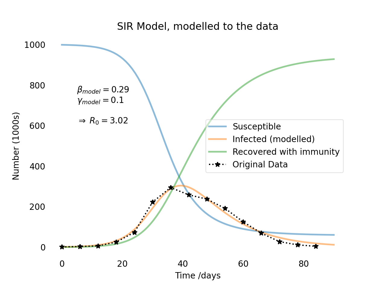 The SIR model with fit to the data.
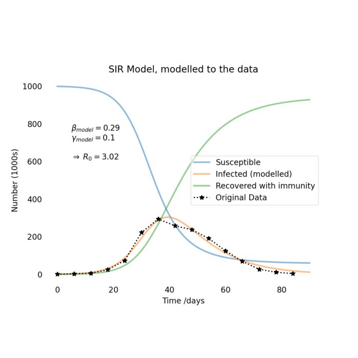
As we can see, the model fits the data quite well. The modelled parameters are $\beta = 0.29$ and $\gamma = 0.1$, which gives us a basic reproduction number of $R_0 = 3.02$. This means that each infected person will infect 3.02 other people on average. This is a relatively high number, which explains why the number of infected people increases so rapidly in the beginning. However, the number of infected people will eventually decrease as more and more people recover and become immune to the disease.
Conclusion
The SIR model provides a valuable framework for understanding the spread and dynamics of epidemics. By dividing the population into susceptible, infectious, and recovered compartments, this model allows us to explore the effects of contact rate and recovery rate on disease transmission. Through the mathematical equations of the SIR model and Python simulations, we can gain insights into the trajectory of an epidemic and estimate key parameters like $\beta$ and $\gamma$. These insights play a crucial role in formulating effective public health measures and making informed decisions in managing the spread of infectious diseases.
The entire code used in this post is available in this GitHub repositoryꜛ.
If you have any questions or suggestions, feel free to leave a comment below.

comments