Introduction to dimensionality reduction in neuroscience
In modern neuroscience, high-dimensional datasets are becoming more common as various experimental methods allow for the simultaneous collection of diverse types of data. These include behavioral recordings, such as multiple videos capturing different body parts, audio recordings, interactions with test devices, and various sensor data. Additionally, neural recordings such as electrophysiology, calcium imaging, or functional MRI (fMRI) are often collected alongside this behavioral data. The result is a complex, multi-dimensional dataset that can be challenging to analyze and interpret.
The primary goal of dimensionality reduction is to simplify this multi-dimensional data, identifying a lower-dimensional representation that preserves the most essential information. By reducing the number of dimensions, or features, the data becomes easier to visualize, cluster, and analyze, while still retaining its core structure and patterns. Dimensionality reduction techniques, such as PCA, t-SNE, UMAP, and autoencoders, are frequently used to reveal latent variables—hidden factors that underlie the observed neural activity or behavior. Once the data is reduced in dimensionality, it can be used for tasks such as visualization, detecting patterns, or applying clustering algorithms.
Why is dimensionality reduction important in neuroscience?
Neuroscience research frequently generates complex, high-dimensional datasets, which can include:
- Neural recordings: These datasets involve spiking activity from neurons recorded over time, using methods like Neuropixels probes or calcium imaging (two- or three-photon imaging), sometimes from thousands of neurons simultaneously.
- RNA sequencing (RNASeq): RNASeq generates gene expression profiles of individual cells, often capturing thousands of genes for each cell.
- Multi-modal experiments: Multi-modal datasets combine different types of measurements, such as electrophysiology, behavior recordings, and imaging data, collected simultaneously.
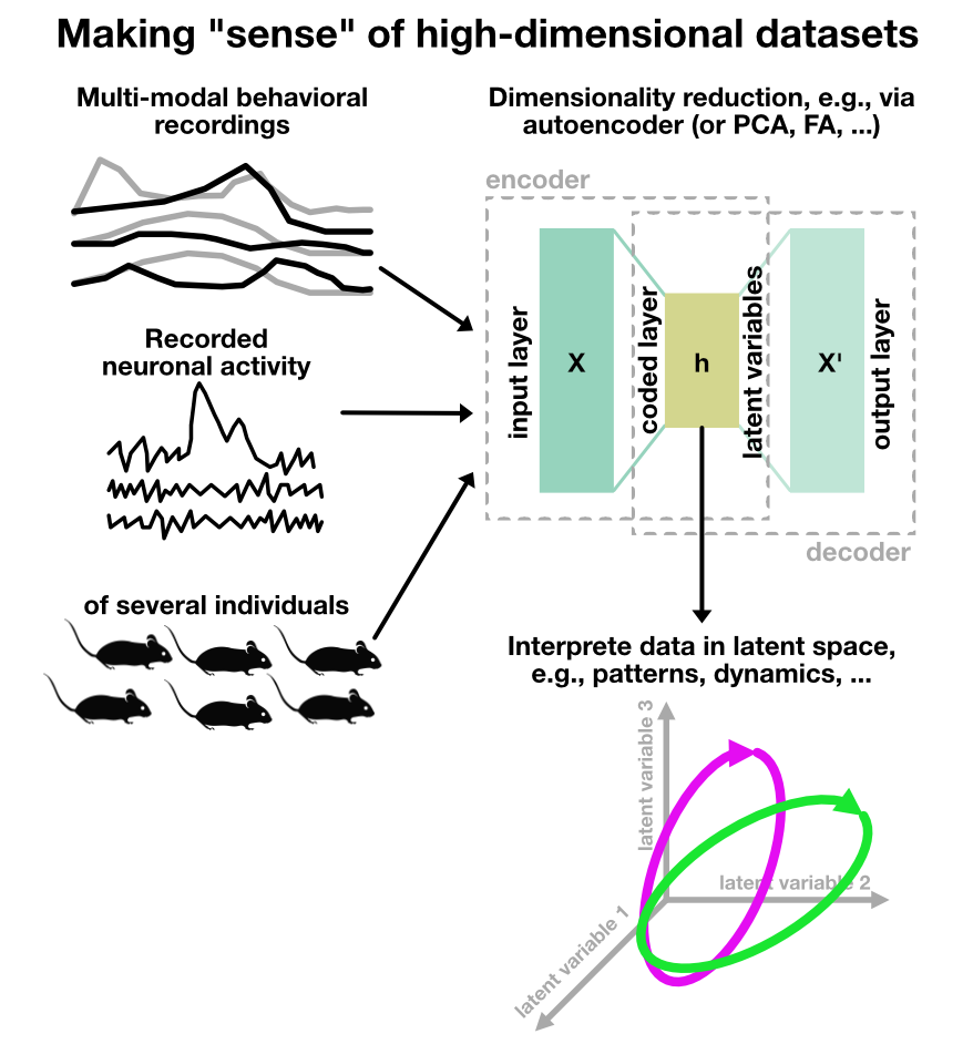
 Illustration of dimensionality reduction in neuroscience. In state-of-the-art experiments, various different measurements are taken simultaneously, ranging from behavioral recordings in a multi-modal manner (e.g., multiple videos from different body parts, audio, interaction with test devices, and other sensor data) and neural recordings (e.g., electrophysiology, calcium imaging, or fMRI). Thus, a high-dimensional dataset is generated. The aim of dimensionality reduction is to find a lower-dimensional representation of this multi-dimensional data that captures the essential information for further analysis. This can be achieved by various techniques, such as PCA, t-SNE, UMAP, or autoencoders, revealing latent variables that govern the behavior and neural activity. The reduced data can then be used for visualization, clustering, or further analysis.
Challenges
The analysis of high-dimensional data poses several challenges:
- Curse of dimensionality: As the number of dimensions increases, the data becomes sparse, and the relationships between data points become harder to interpret. Many features may also be irrelevant or noisy, complicating the analysis.
- Redundancy: In high-dimensional datasets, many features may be correlated or redundant. For instance, firing rates from different neurons or gene expression levels across related genes may convey similar information, making it difficult to discern meaningful patterns.
Benefits of dimensionality reduction
Dimensionality reduction helps tackle these challenges by condensing high-dimensional datasets into lower-dimensional forms while preserving important relationships. The key benefits include:
- Visualization: By reducing high-dimensional data to 2D or 3D, dimensionality reduction makes the data more interpretable for human analysis and exploration.
-
Pattern recognition: It aids in identifying underlying structures, such as activity patterns in neurons or clusters of similar cells in RNASeq data.
- Noise reduction: Dimensionality reduction can help eliminate noise and irrelevant variations in the data, making the core features more apparent.
Applications of dimensionality reduction in neuroscience
Neural Recordings
In experiments where electrophysiology or calcium imaging captures neural activity, we need to analyze the simultaneous activity of large neural populations. Dimensionality reduction can help uncover population-level dynamics, identify neural states, and detect activity patterns that relate to behavior or external stimuli.
For example: A spike train data from thousands of neurons can be reduced to reveal latent variables that govern the overall neural activity, simplifying complex datasets into meaningful representations.
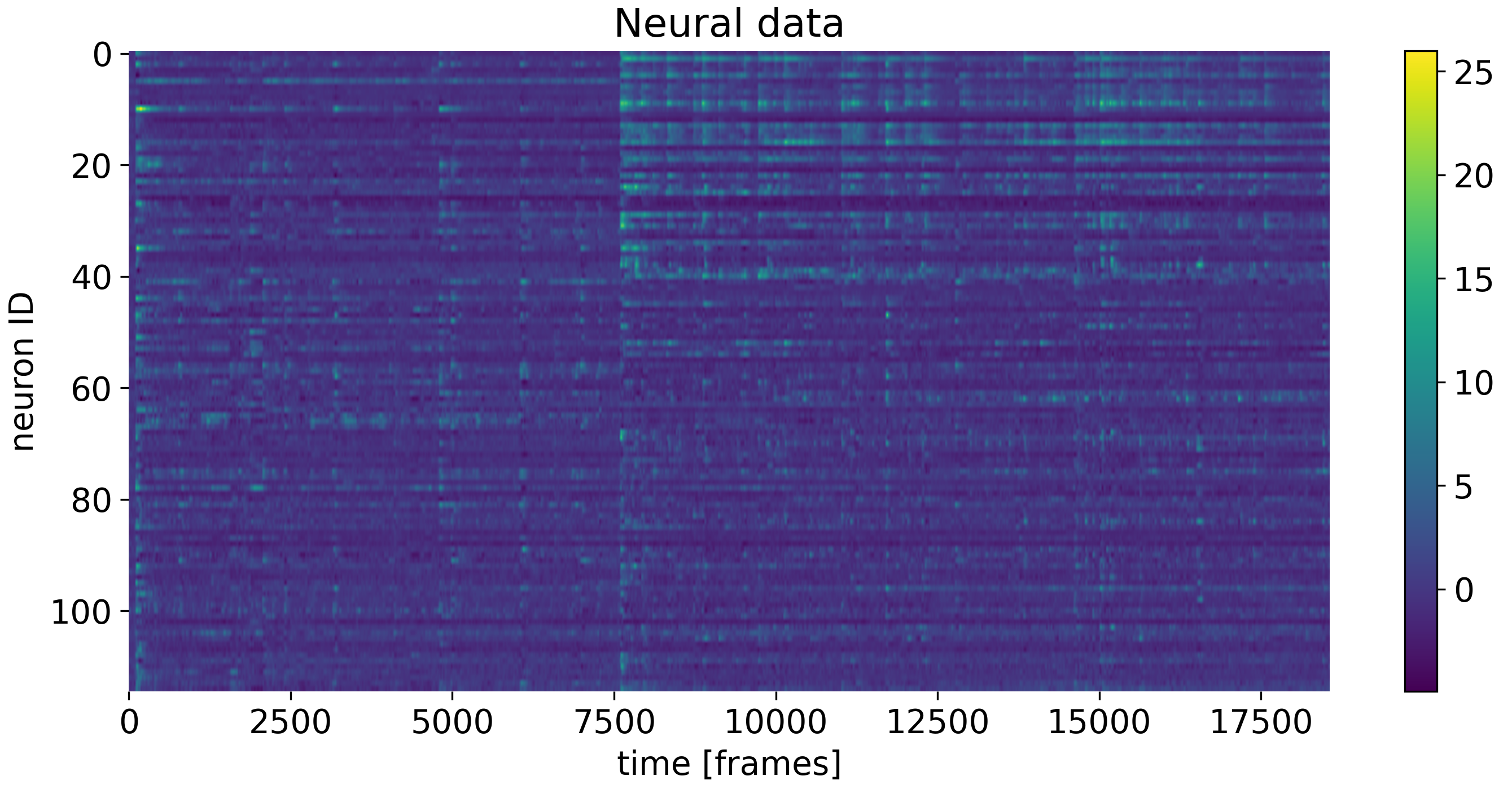
 Example dataset of neural data of $\gt$100 recorded neurons of a mouse as a function of time.
RNASeq Data
In single-cell RNA sequencing (scRNASeq), we measure the expression levels of thousands of genes across many individual cells. Dimensionality reduction techniques are crucial for:
- Identifying cell types and subtypes by clustering cells with similar gene expression profiles.
- Visualizing gene expression trends to understand how groups of genes behave across cells.
- Clustering cells into groups based on their genetic profiles, helping to identify biological processes or conditions.
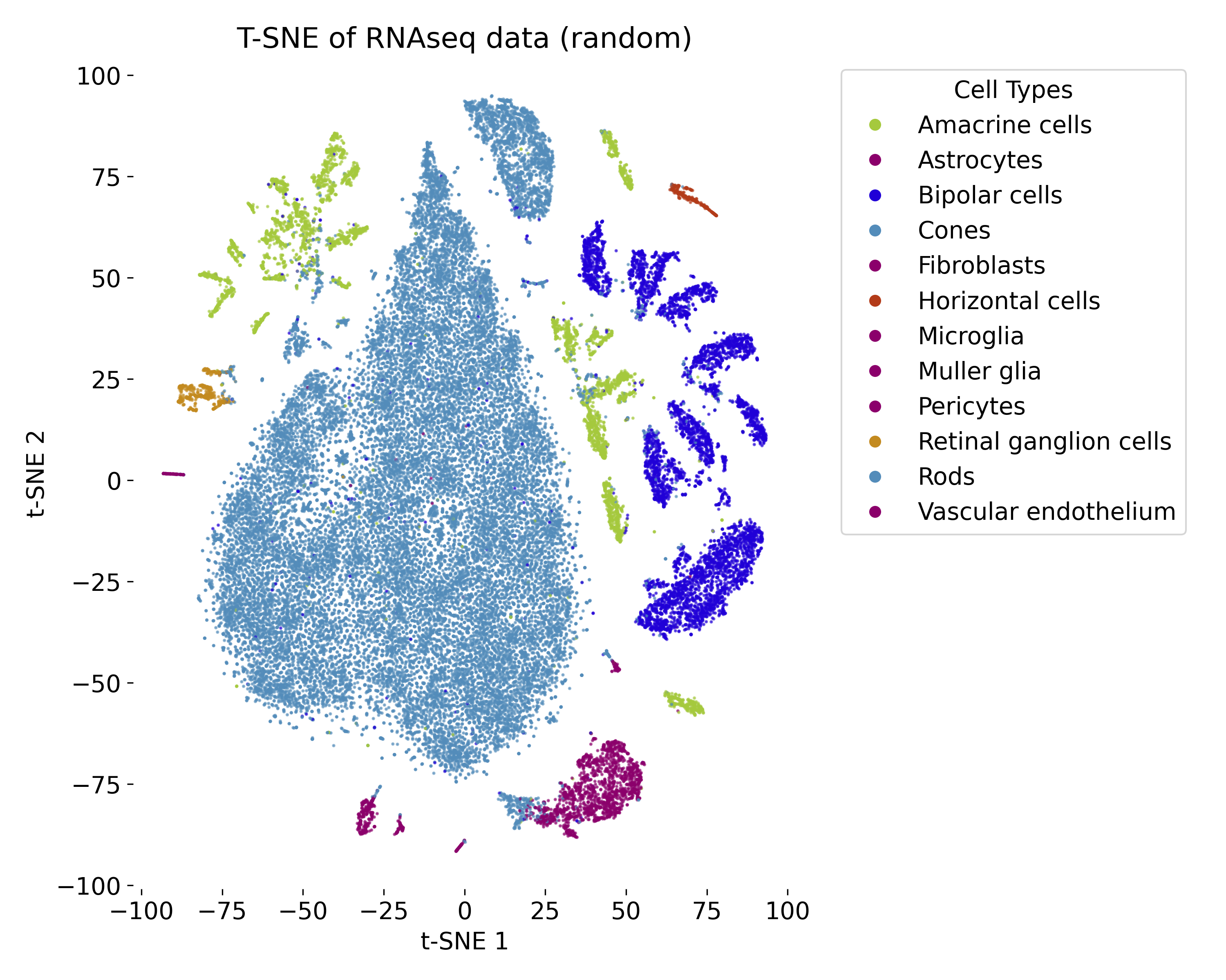
 t-SNE plot of the RNAseq dataset of 48,000 cells.
Multi-modal Experiments
In multi-modal neuroscience experiments, we combine neural recordings, behavioral data, and imaging data. Dimensionality reduction plays a central role in:
- Integrating data across modalities by finding shared latent variables or factors linking neural activity with behavior.
- Exploring relationships between different types of measurements, such as how neural activity correlates with movement or external stimuli.
- Discovering latent patterns in multi-modal datasets that reflect underlying neural processes or behavioral strategies.
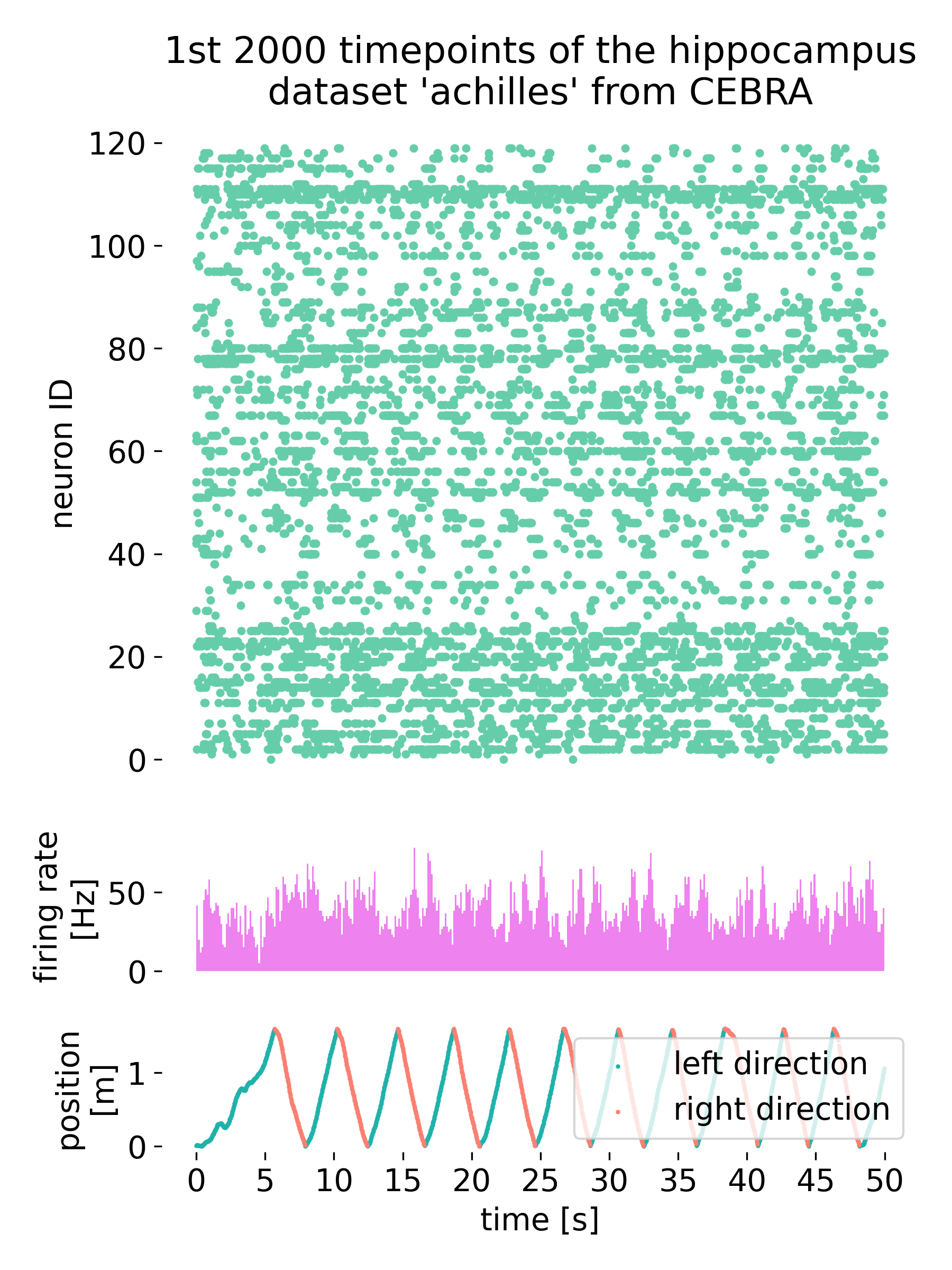
 Neural data (top) of $\gt$100 recorded cells of a mouse and its average firing rate (middle) as a function of time. Simultaneously, the mouse performs a behavior (bottom).
Techniques for dimensionality reduction
Principal Component Analysis (PCA)
PCA is one of the most widely used linear dimensionality reduction techniques. It projects the high-dimensional data onto a smaller number of principal components that capture the greatest variance in the dataset. PCA is often the first step in exploring high-dimensional data, providing a quick way to understand the structure of the data.
Autoencoders
Autoencoders are neural networks designed to learn a compact, latent representation of the input data. Autoencoders are particularly useful for compressing high-dimensional data, such as neural recordings or gene expression data, into a lower-dimensional space for further analysis. The learned latent space can reveal hidden factors or patterns in the data.
Clustering
Clustering algorithms, such as k-means or DBSCAN, can be used in conjunction with dimensionality reduction techniques to identify groups or clusters of similar data points. Clustering helps uncover patterns in the data and can be applied to both high-dimensional and reduced-dimensional datasets.
t-SNE (t-distributed Stochastic Neighbor Embedding)
t-SNE is a non-linear dimensionality reduction technique specifically designed for visualizing high-dimensional data in low-dimensional spaces (usually 2D or 3D). It is commonly used in scRNASeq data analysis and neural population activity analysis because it effectively captures local clusters and relationships. However, it can sometimes struggle to preserve global structures in the data.
UMAP (Uniform Manifold Approximation and Projection)
UMAP is another non-linear dimensionality reduction technique that improves upon t-SNE by preserving both local and global structures. UMAP is often used for visualizing cell populations, neural activity patterns, and integrating multimodal datasets. It is faster than t-SNE and scales better with large datasets.
Course format
This intensive 1.5-day course will consist of
- Lectures: Each topic will be introduced with a (short) theoretical background and relevant mathematical foundations. However, we focus on the practical application of each method.
- Hands-on sessions: Practical exercises using Python and popular libraries (such as scikit-learn and PyTorch) to implement and experiment with each method.
Prerequisites
- Basic knowledge of Python programming, usage of conda or pip for package management, usage of GitHub, and familiarity with Jupyter notebooks.
- Your own laptop with the a running Python environment (e.g., miniconda or Anaconda).
- Familiarity with fundamental concepts in machine learning and neuroscience is beneficial but not required.
Who should attend?
- Neuroscientists and researchers interested in applying machine learning techniques to their data.
- Data scientists and machine learning practitioners looking to specialize in neuroscience applications.
- Graduate students and professionals in related fields seeking practical skills in dimensionality reduction.
Topics covered
- Principal Component Analysis (PCA)
- Clustering
- t-Distributed Stochastic Neighbor Embedding (t-SNE)
- Uniform Manifold Approximation and Projection (UMAP)
- Autoencoders (AE)
- Varietional Autoencoders (VAE)
Time schedule
Our course will be structured as follows:
- Day 1: Introduction, PCA, Clustering, t-SNE, UMAP
- 9:00 AM - 9:30 AM: Welcome and introduction to dimensionality reduction
- 9:30 AM - 11:00 AM: Principal Component Analysis (PCA)
- 9:30 AM - 10:00 AM: PCA introduction
- 10:00 AM - 10:45 AM: PCA hands-on
- 10:45 AM - 11:00 AM: PCA hands-on discussion
- 11:00 AM - 11:15 AM: Break
- 11:15 AM - 12:45 PM: Clustering
- 11:15 AM - 11:45 AM: Clustering introduction
- 11:45 AM - 12:30 PM: Clustering hands-on
- 12:30 PM - 1:30 PM: Lunch Break
- 1:30 PM - 2:00 PM: Clustering hands-on discussion
- 2:00 PM - 3:30 PM: t-Distributed Stochastic Neighbor Embedding (t-SNE)
- 2:00 PM - 2:30 PM: t-SNE introduction
- 2:30 PM - 3:15 PM: t-SNE hands-on
- 3:15 PM - 3:30 PM: t-SNE hands-on discussion
- 3:30 PM - 3:45 PM: Break
- 3:45 PM - 4:45 PM: Uniform Manifold Approximation and Projection (UMAP)
- 3:45 PM - 4:15 PM: UMAP introduction
- 4:15 PM - 4:30 PM: UMAP hands-on
- 4:30 PM - 4:45 PM: UMAP hands-on discussion
- 4:45 PM - 5:00 PM: Wrap-up day 1 and Q&A
- Day 2: Autoencoders
- 9:00 AM - 10:30 AM: Autoencoders (1)
- 9:00 AM - 10:30 AM: Autoencoders introduction
- 10:30 AM - 11:15 AM: Autoencoders hands-on (exercise 1)
- 11:15 AM - 11:30 AM: Break
- 11:30 AM - 12:00 PM: Autoencoders (2)
- 11:30 AM - 12:00 PM: Autoencoders hands-on (exercise 1) discussion
- 12:00 PM - 1:00 PM: Lunch Break
- 1:00 PM - 2:00 PM: Autoencoders (2)
- 1:00 PM - 1:45 PM: Autoencoders hands-on (exercise 2)
- 1:45 PM - 2:00 PM: Autoencoders hands-on (exercise 2) discussion
- 2:00 PM - 2:15 PM: Coffee Break
- 2:15 PM - 4:00 PM: Variational Autoencoders (VAE)
- 2:15 PM - 2:45 PM: VAE introduction
- 2:45 PM - 3:30 PM: VAE hands-on
- 3:30 PM - 3:45 PM: VAE hands-on discussion
- 3:45 PM - 4:00 PM: Final discussion and course wrap-up
- 9:00 AM - 10:30 AM: Autoencoders (1)