Bienenstock-Cooper-Munro (BCM) rule

The Bienenstock-Cooper-Munro (BCM) rule is a cornerstone in theoretical neuroscience, offering a comprehensive framework for understanding synaptic plasticity – the process by which connections between neurons are strengthened or weakened over time. Since its introduction in 1982ꜛ, the BCM rule has provided critical insights into the mechanisms of learning and memory formation in the brain. In this post, we briefly explore and discuss the BCM rule, its theoretical foundations, mathematical formulations, and implications for neural plasticity.

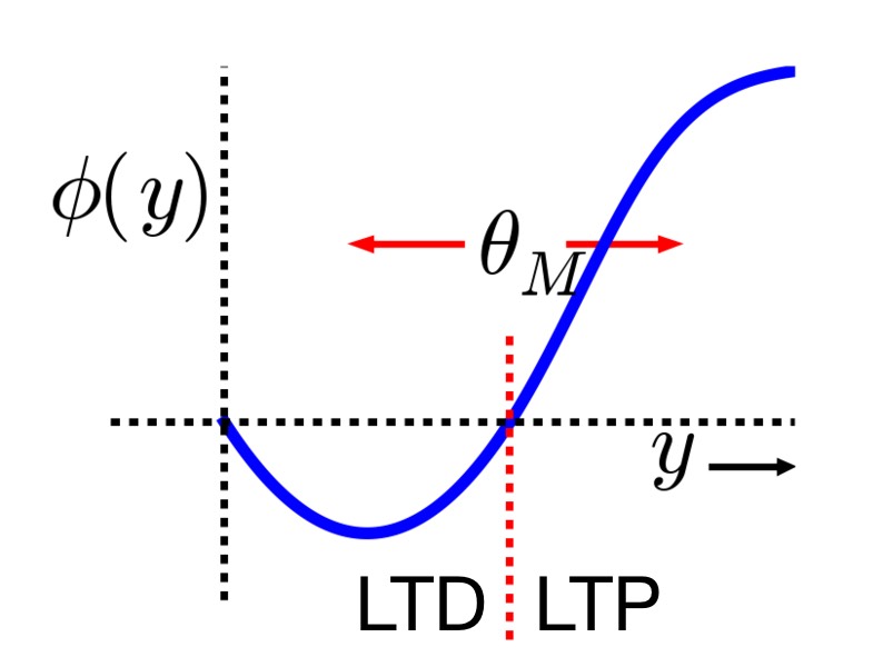
Relationship between postsynaptic activity $y$ and the modification function $\phi(y)$ (blue line), which is dependent on the dynamic threshold $\theta_M$ (red dashed line). Two distinct regimes can be identified: for $y < \theta_M$ (left of the red dashed line), the modification function is negative, leading to LTD (the synaptic strength decreases in this region), while for $y > \theta_M$ (right of the red dashed line), the modification function is positive, leading to LTP (the synaptic strength increases in this region). Image source (modified): scholarpedia.orgꜛ.

Theoretical foundations of the BCM Rule

The BCM rule was proposed by Elie Bienenstock, Leon Cooper, and Paul Munroꜛ to address how neurons in the visual cortex develop selectivity to specific patterns, such as orientation or spatial frequency. The rule posits that synaptic changes depend not only on the immediate activity of the pre- and postsynaptic neurons but also on the history of postsynaptic activity. This historical dependence introduces a sliding threshold that determines whether synaptic activity leads to long-term potentiation (LTP) or long-term depression (LTD). LTP refers to the strengthening of synaptic connections, while LTD refers to the weakening of synaptic connections. These processes are essential for learning and memory formation in the brain. In LTP, repeated activation of a synapse leads to an increase in synaptic strength, making it more likely to fire in response to a given input. In contrast, LTD weakens synaptic connections, reducing the likelihood of firing. We will further explain LTP and LTD in the next post.

The core idea is that there is a dynamic threshold for synaptic modification, $\theta_M$, which adjusts based on the postsynaptic activity. Synaptic strength increases (LTP) when the postsynaptic activity $y$ exceeds this threshold, and decreases (LTD) when it falls below it. Importantly, the dynamic threshold itself changes in response to the average postsynaptic activity, $\langle y \rangle$, allowing the system to adapt to different activity levels.

By incorporating the dynamic threshold into the learning process, the BCM rule captures the interplay between neural activity and synaptic plasticity, providing a mechanism for how neurons develop selectivity and maintain stability over time.

Mathematical formulation

The BCM rule can be mathematically described using a few key equations. Let $x_i$ be the presynaptic activity of the $i$-th neuron, $y$ be the postsynaptic activity,

\[y = \sum_i w_i x_i\]

and $w_i$ be the corresponding synaptic weight.

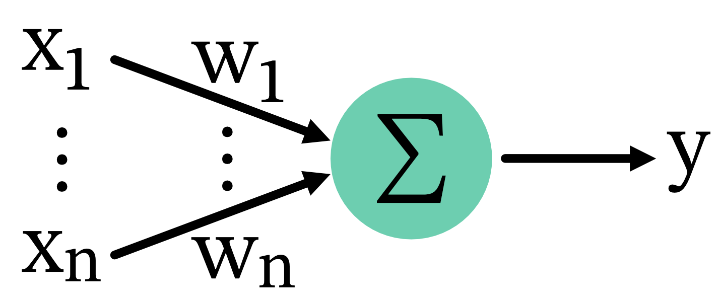
Connectivity scheme: Presynamtic neurons $x_i$ project to a postsynaptic neuron $y$ with corresponding synaptic weights $w_i$. The postsynaptic activity $y$ is the sum of the products of presynaptic activities and synaptic weights.

The change in synaptic weight, ${dw_i}/{dt}$, is given by:

\[\frac{dw_i}{dt} = \eta \cdot y \cdot (y - \theta_M) \cdot x_i\]

Here, $\eta$ is a learning rate constant, and $\theta_M$ is the modification threshold. The threshold $\theta_M$ itself is a function of the time-averaged postsynaptic activity, $\langle y \rangle$:

\[\theta_M = \phi(\langle y \rangle)\]

where $\phi(\langle y \rangle)$ is a monotonically increasing function, typically represented as:

\[\phi(\langle y \rangle) = \langle y \rangle^p\]

with $p > 1$.

To provide a complete mathematical model, we consider the dynamics of the time-averaged postsynaptic activity, $\langle y \rangle$, which evolves according to:

\[\tau \frac{d \langle y \rangle}{dt} = - \langle y \rangle + y\]

where $\tau$ is a time constant.

In the literature, various extensions and refinements of the BCM rule have been proposed, incorporating additional factors such as metaplasticity, homeostatic regulation, and network interactions. These modifications aim to capture the complex interplay of factors influencing synaptic plasticity in neural circuits.

A variant of the BCM rule adds a weight decay term $-\epsilon w_i$ to the Hebbian-like term $y \cdot (y - \theta_M) \cdot x_i$ instead of multiplying it by the learning rate, allowing for a more nuanced regulation of synaptic changes over time:

\[\frac{dw_i}{dt} = y \cdot (y - \theta_M) \cdot x_i - \epsilon w_i\]

The weight decay term acts to stabilize the weight, preventing it from growing indefinitely. This modified BCM rule is different from the previous BCM formulation in that it explicitly includes a mechanism to reduce the synaptic weight over time, proportional to its current value. This is a common modification in neural network models to ensure weights do not grow without bound and to introduce a form of weight regularization.

Implications and predictions of the BCM rule

The BCM rule offers several significant implications for synaptic plasticity:

Stability of synaptic weights:

The classical Hebbian learning rule can be expressed as: $\Delta w_i = \eta \cdot x_i \cdot y$, where $\Delta w_i$ is the change in synaptic weight, $\eta$ is again the learning rate, and $x_i$ and $y$ are the presynaptic and postsynaptic activity, respectively. Hebbian learning tends to lead to runaway potentiation, where synaptic weights increase without bound. This is because the positive feedback loop of strengthening synapses leads to further increases in activity, which in turn strengthens the synapses even more. The introduction of the sliding threshold $\theta_M$ in the BCM rule addresses this issue by providing a mechanism for homeostatic regulation in the neural network as it ensures that synaptic weights remain stable over time. For example, if a neuron experiences high activity, $\theta_M$ increases, making it less likely for further potentiation.

Synaptic competition and selectivity:

Classical Hebbian learning does not inherently promote competition among synapses. Without additional mechanisms, such as normalization or competition, all synapses could potentially increase together, which is not biologically realistic. In contrast, the BCM rule naturally leads to synaptic competition and selectivity. Synapses receiving correlated inputs and, thus, frequently having their activity levels above $\theta_M$ are strengthened, while those receiving uncorrelated inputs (i.e., less active synapses) are weakened. This mechanism explains the development of feature selectivity, such as orientation selectivity in visual cortex neurons.

Activity-dependent plasticity:

By depending on the time-averaged postsynaptic activity, $\langle y \rangle$, the BCM rule adapts to varying activity regimes. This supports both homeostatic regulation, where synapses adjust to maintain overall stability, and experience-dependent plasticity, where synapses change based on specific patterns of activity. In contrast, classical Hebbian learning is purely activity-dependent and does not consider the historical activity of the neuron. This can lead to synapses becoming overly strong if there is sustained high activity, or overly weak if there is sustained low activity.

Bidirectional plasticity

This point is an implication of the previous ones, but still worth mentioning. Classical Hebbian learning primarily accounts for potentiation (strengthening) of synapses. Variants like anti-Hebbian learning are required to explain synaptic weakening (depression). The BCM rule inherently supports bidirectional plasticity. When the postsynaptic activity $y$ is above the threshold $\theta_M$, LTP (long-term potentiation) occurs. When $y$ is below $\theta_M$, LTD (long-term depression) occurs. This bidirectional nature makes the BCM rule more versatile and better suited to modeling biological synaptic plasticity.

Python example

To illustrate the dynamics of the BCM rule, consider a simple computational model with two synapses receiving inputs $x_1$ and $x_2$. The postsynaptic activity $y$ is given by:

\[y = w_1 x_1 + w_2 x_2\]

The synaptic weights $w_1$ and $w_2$ are updated according to the BCM rule:

\[\begin{align*} \Delta w_1 &= \eta \cdot y \cdot (y - \theta_M) \cdot x_1 \\ \Delta w_2 &= \eta \cdot y \cdot (y - \theta_M) \cdot x_2 \end{align*}\]

By simulating this system over time, we can observe the evolution of synaptic weights and the development of selectivity. For instance, if $x_1$ and $x_2$ represent different sensory inputs, the synapse corresponding to the more frequently activated input will strengthen, demonstrating the competitive nature of synaptic plasticity under the BCM rule.

Let’s transfer this model into a simple Python script to simulate the synaptic weight changes over time. We will consider the two-synapse system and simulate the system over multiple time steps to observe how the synaptic weights evolve based on the postsynaptic activity $y$:

import os
import numpy as np
import matplotlib.pyplot as plt

# set global properties for all plots:
plt.rcParams.update({'font.size': 12})
plt.rcParams["axes.spines.top"]    = False
plt.rcParams["axes.spines.bottom"] = False
plt.rcParams["axes.spines.left"]   = False
plt.rcParams["axes.spines.right"]  = False

# for reproducibility:
np.random.seed(1)

# define parameters:
eta             = 0.01  # learning rate
tau             = 100.0  # time constant for averaging postsynaptic activity
epsilon         = 0.001  # decay rate (only used if decay term is included)
simulation_time = 500  # total simulation time in ms
time_step       = 1  # time step for the simulation in ms
p               = 2  # exponent for the sliding threshold function

# initialize synaptic weights and inputs:
w  = np.array([0.5, 0.5])  # Initial synaptic weights
x1 = np.random.rand(simulation_time)  # Presynaptic input 1
x2 = np.random.rand(simulation_time)  # Presynaptic input 2
inputs = np.vstack((x1, x2))

# initialize variables for storing results:
y       = np.zeros(simulation_time)
theta_M = np.zeros(simulation_time)
avg_y   = 0  # initial average postsynaptic activity
w_history = np.zeros((simulation_time, 2))  # to store synaptic weights over time

# simulation loop:
for t in range(simulation_time):
    # compute postsynaptic activity:
    y[t] = np.dot(w, inputs[:, t])
    
    # update average postsynaptic activity:
    avg_y = avg_y + (y[t] - avg_y) / tau
    
    # update the sliding threshold:
    theta_M[t] = avg_y ** p
    
    # update synaptic weights according to the BCM rule:
    delta_w = eta * y[t] * (y[t] - theta_M[t]) * inputs[:, t]
    # uncomment the following line to include weight decay:
    # delta_w = eta * y[t] * (y[t] - theta_M[t]) * inputs[:, t] - epsilon * w
    w += delta_w
    
    # ensure weights remain within a reasonable range:
    w = np.clip(w, 0, 1)
    
    # store synaptic weights:
    w_history[t] = w

# plotting the results:
plt.figure(figsize=(6, 7))

# Plot synaptic weights
plt.subplot(2, 1, 1)
plt.plot(w_history[:, 0], label='weight 1')
plt.plot(w_history[:, 1], label='weight 2')
plt.xlabel('time [ms]')
plt.ylabel('synaptic weight')
plt.title('Evolution of synaptic weights')
plt.legend()

# Plot postsynaptic activity and sliding threshold
plt.subplot(2, 1, 2)
plt.plot(y, label='postsynaptic activity')
plt.plot(theta_M, label='sliding threshold', linestyle='--')
plt.xlabel('time [ms]')
plt.ylabel('activity / threshold')
plt.title('Postsynaptic activity and sliding threshold')
plt.legend()

plt.tight_layout()
plt.show()

Here is the corresponding output of simulation for the default BCM rule:

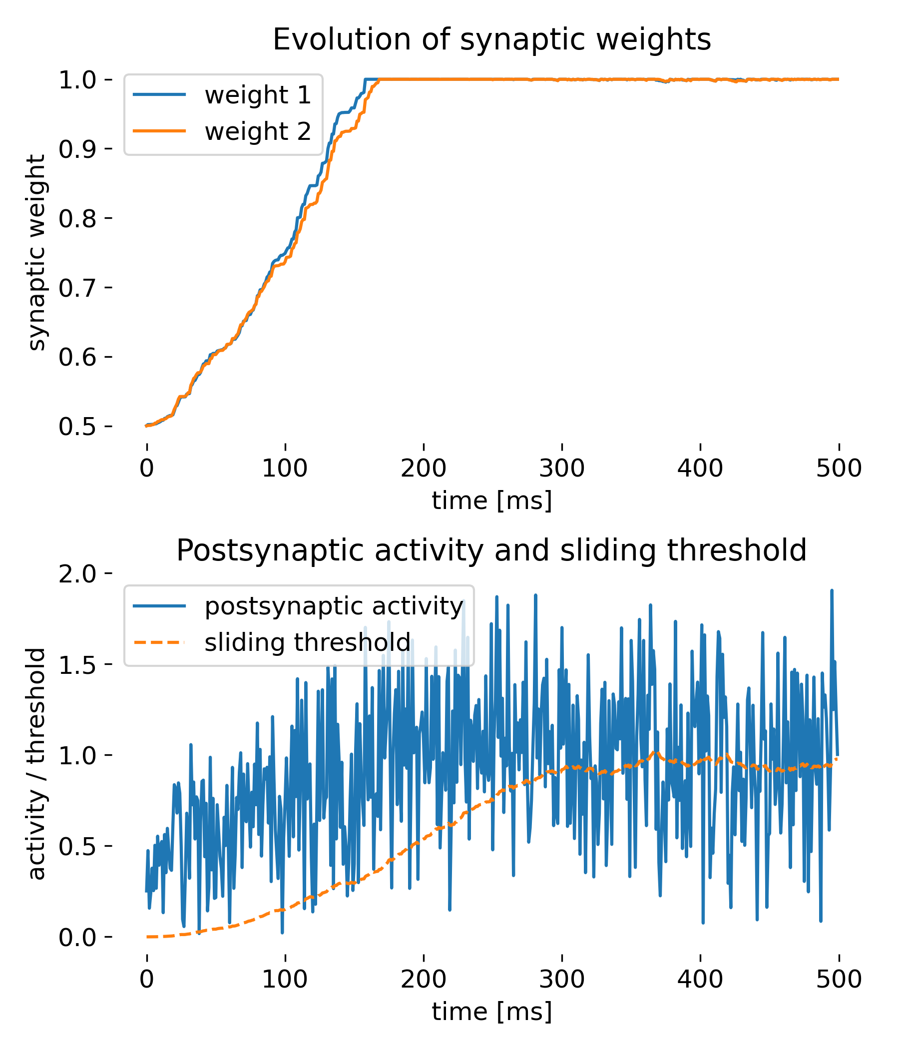
Simulation of two presynaptic inputs and one postsynaptic neuron. The top plot shows the evolution of synaptic weights over time, while the bottom plot displays the postsynaptic activity and the sliding threshold. The synaptic weights adapt to the inputs, demonstrating the competitive nature of synaptic plasticity under the BCM rule.

The top plot shows the evolution of synaptic weights $w_1$ and $w_2$ over time. Initially, both weights increase steadily. After reaching a certain time point, they saturate and remain constant at the maximum value of 1. This behavior is expected under the BCM rule, where the weights increase when the postsynaptic activity $y$ is greater than the sliding threshold $\theta_M$. The saturation indicates that the inputs were sufficiently correlated or frequent to push the weights to their upper limit. The weights being clipped at 1 is a safeguard to prevent unbounded growth as discussed before.

The bottom plot shows the postsynaptic activity $y$ and the sliding threshold $\theta_M$ over time. The postsynaptic activity $y$ increased over time, but fluctuates widely, whereas the sliding threshold $\theta_M$ increases more gradually. The wide fluctuations in $y$ reflect the variability in presynaptic inputs. The gradual increase in $\theta_M$ is indicative of the time-averaging process of the postsynaptic activity, capturing the overall increase in activity over time. This shows how the BCM rule adapts the threshold to maintain stability and avoid runaway potentiation.

Thus, all core features of the BCM rule are demonstrated by this simple simulation:

• Dynamic threshold adaptation: The sliding threshold $\theta_M$ adapts based on the average postsynaptic activity, which is a core aspect of the BCM rule.
• Synaptic plasticity mechanism: The change in synaptic weights based on the relationship between postsynaptic activity and the sliding threshold demonstrates the core plasticity mechanism of the BCM rule.
• Stability of weights: The saturation of weights at a maximum value showcases the stability mechanism of the BCM rule, preventing unbounded growth.

In case you want to simulate the BCM rules including the weight decay term, simply change the update rule:

# update synaptic weights according to the BCM rule:
#delta_w = eta * y[t] * (y[t] - theta_M[t]) * inputs[:, t]
# uncomment the following line to include weight decay:
delta_w = eta * y[t] * (y[t] - theta_M[t]) * inputs[:, t] - epsilon * w

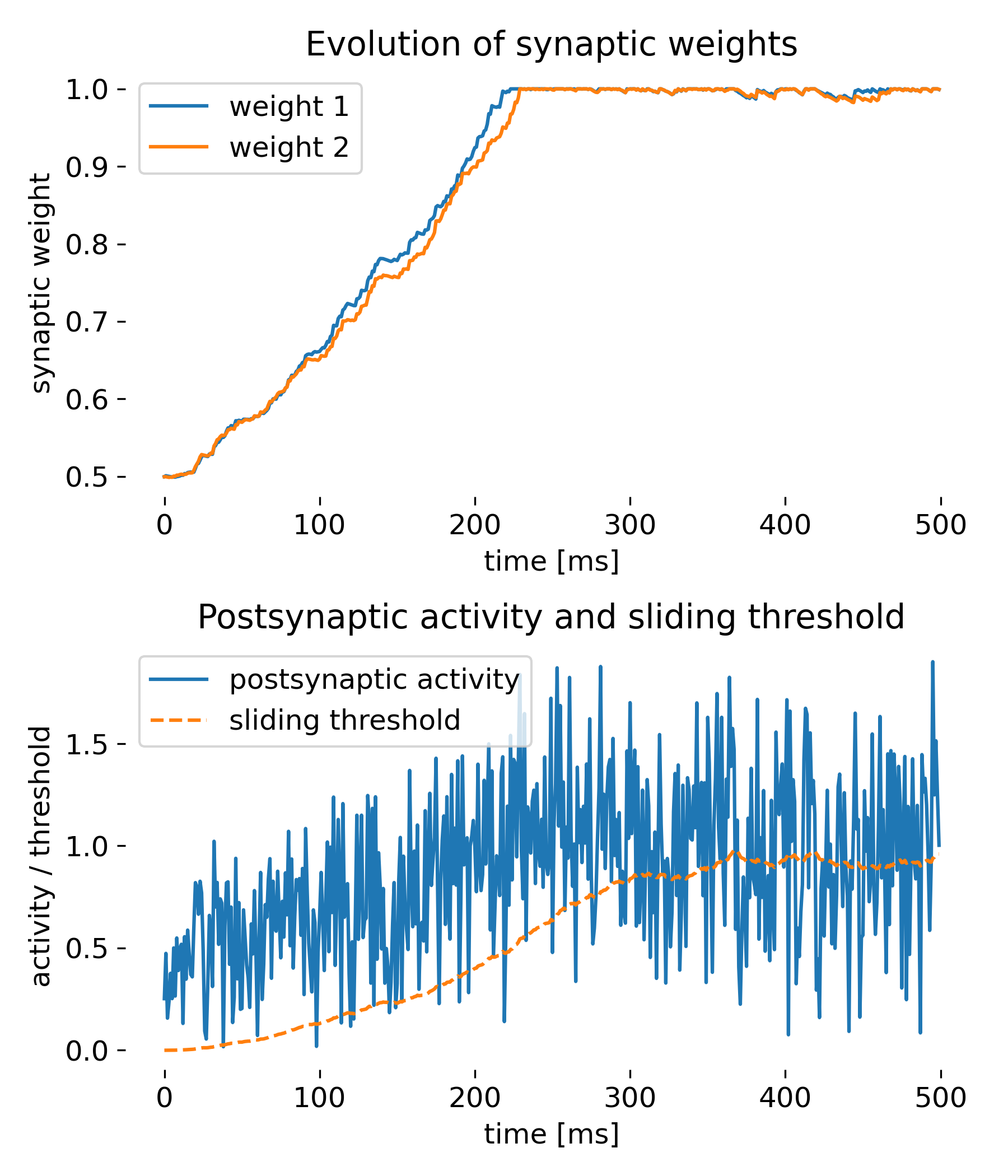
Same simulation as before, but with the weight decay term included.

While the synaptic weights approach saturation a bit slower this time, the simulation shows that the weight decay term is also able to stabilize the weights over time, preventing them from growing indefinitely. This is a common strategy in neural network models to ensure that weights do not become too large and to introduce a form of regularization.

Experimental Evidence and Applications

The BCM rule has received substantial experimental support. Studies on visual cortex plasticity have demonstrated that neurons adapt their response properties based on sensory experience, consistent with the predictions of the BCM theory. Additionally, the rule has been applied to various neural circuits, providing insights into the mechanisms of learning and memory across different brain regions.

Study on visual cortex plasticity – For instance, Udeigwe et al. 2017ꜛ have demonstrated that the BCM rule can model how neurons in the visual cortex adapt their response properties based on sensory experience. Specifically, studies such as Lian et al. 2021ꜛ using natural images as stimuli have shown that neurons can develop receptive fields similar to those of simple cells in the visual cortex through a competitive synaptic learning process driven by the BCM rule. These findings highlight the rule’s ability to explain the development of stimulus selectivity in the visual cortex.

Empirical evidence for bidirectional plasticity – Experimental studies have confirmed the bidirectional nature of synaptic plasticity as predicted by the BCM rule. For example, experiments by Dudek and Bear (1992)ꜛ and Mulkey and Malenka (1992)ꜛ demonstrated that high-frequency stimulation induces LTP, while low-frequency stimulation leads to LTD in hippocampal neurons. These results are consistent with the BCM rule’s prediction that the direction and magnitude of synaptic changes depend on postsynaptic activity (Shouval et al. 2010ꜛ).

Modeling experience-dependent plasticity – The BCM theory has been successfully applied to model various aspects of experience-dependent plasticity in the visual cortex. Studies have shown that under different rearing conditions, such as dark rearing, the BCM rule can account for the observed changes in synaptic strength and neuronal selectivity. Dark rearing, where animals (typically rodents) are raised in complete darkness for extended periods, is an experimental approach to study how visual deprivation affects cortical plasticity. The BCM theory predicts that in such conditions, the threshold for LTP would shift downward due to the overall reduced neuronal activity in the absence of visual stimuli. This decreased threshold makes it easier for synapses to undergo potentiation in response to any remaining input, but may impair the proper tuning of synaptic connections. When normal vision is restored after dark rearing, this shift in the LTP threshold can lead to impaired visual cortical plasticity, as the system is not adequately primed to adjust to the new sensory environment. These findings are supported by studies such as Rittenhouse et al. (1999)ꜛ and Bear et al. (1987)ꜛ, which demonstrate that dark rearing leads to significant changes in the cortical representation of visual stimuli.

Astrocytic modulation of plasticity – Recent research by Squadrani et al. (2024)ꜛ has further advanced the experimental justification for the BCM rule by demonstrating the crucial role of astrocytes in synaptic plasticity during cognitive tasks such as reversal learning. In their study, astrocytes were shown to enhance the plasticity response, acting as key modulators of synaptic strength by regulating the activity of neurons. Their findings suggest that astrocytic signaling can influence the threshold dynamics predicted by the BCM rule, adjusting the balance between LTP and LTD in a manner dependent on the cognitive demands of the task. This not only supports the BCM model’s applicability in more complex, behaviorally relevant settings but also emphasizes the importance of glial cells in synaptic plasticity, extending the original neuron-centric framework of the BCM theory to incorporate neuron-astrocyte interactions.

Conclusion

The BCM rule is a fundamental theory in neuroscience, providing a robust framework for understanding synaptic plasticity. Its mathematical formulation captures the dynamic nature of synaptic changes, incorporating both immediate neural activity and historical context. By explaining how neurons develop selectivity and maintain stability and supported by experimental evidence, the BCM theory continues to provide valuable insights into the mechanisms behind learning and memory formation, making it a fundamental tool for advancing research in neural plasticity.

The complete code used in this blog post is available in this Github repositoryꜛ (bcm_rule.py and bcm_rule_with_decay_term.py). Feel free to modify and expand upon it, and share your insights.

References and useful links

• E. L. Bienenstock, L. N. Cooper, P. W. Munro, Theory for the development of neuron selectivity: orientation specificity and binocular interaction in [visual cortex, 1982, Journal of Neuroscience, doi: 10.1523/JNEUROSCI.02-01-00032.1982ꜛ
• Intrator, Cooper, Objective function formulation of the BCM theory of visual cortical plasticity: Statistical connections, stability conditions, 1992, Neural Networks, Vol. 5, Issue 1, pages 3-17, doi: 10.1016/S0893-6080(05)80003-6ꜛ
• Brian S. Blais and Leon Cooper, BCM theory, 2008, Scholarpedia, 3(3):1570, doi: 10.4249/scholarpedia.1570ꜛ
• Lian, Almasi, Grayden, Kameneva, Burkitt, Meffin, Learning receptive field properties of complex cells in V1, 2021, PLOS Computational Biology, Vol. 17, Issue 3, pages e1007957, doi: 10.1371/journal.pcbi.1007957ꜛ
• Udeigwe, Munro, Ermentrout, Emergent Dynamical Properties of the BCM Learning Rule, 2017, The Journal of Mathematical Neuroscience, Vol. 7, Issue 1, pages n/a, doi: 10.1186/s13408-017-0044-6ꜛ
• Shouval, Spike timing dependent plasticity: A consequence of more fundamental learning rules, 2010, Frontiers in Computational Neuroscience, Vol. n/a, Issue n/a, pages n/a, doi: 10.3389/fncom.2010.00019
• Dudek, Bear, Homosynaptic long-term depression in area CA1 of hippocampus and effects of N-methyl-D-aspartate receptor blockade., 1992, Proceedings of the National Academy of Sciences, Vol. 89, Issue 10, pages 4363-4367, doi: 10.1073/pnas.89.10.4363ꜛ
• Mulkey, Malenka, Mechanisms underlying induction of homosynaptic long-term depression in area CA1 of the hippocampus, 1992, Neuron, Vol. 9, Issue 5, pages 967-975, doi: 10.1016/0896-6273(92)90248-cꜛ
• Bear, Cooper, Ebner, A Physiological Basis for a Theory of Synapse Modification, 1987, Science, Vol. 237, Issue 4810, pages 42-48, doi: 10.1126/science.3037696ꜛ
• Rittenhouse, Shouval, Paradiso, Bear, Monocular deprivation induces homosynaptic long-term depression in visual cortex, 1999, Nature, Vol. 397, Issue 6717, pages 347-350, doi: 10.1038/16922ꜛ
• Squadrani, Wert-Carvajal, Müller-Komorowska, Bohmbach, Henneberger, Verzelli, Tchumatchenko, Astrocytes enhance plasticity response during reversal learning, 2024, Communications Biology, Vol. 7, Issue 1, pages n/a, doi: 10.1038/s42003-024-06540-8ꜛ