Olfactory processing via spike-time based computation

August 21, 2024 10 minute read comments

In their work “Simple Networks for Spike-Timing-Based Computation, with Application to Olfactory Processing” from 2003, Brody and Hopfieldꜛ proposed a simple network model for olfactory processing. Brody and Hopfield showed how networks of spiking neurons (SNN) can be used to process temporal information based on computations on the timing of spikes rather than the rate of spikes. This is particularly relevant in the context of olfactory processing, where the timing of spikes in the olfactory bulb is crucial for encoding odor information. In this tutorial, we recapitulate the main concepts of Brody and Hopfield’s network using the NEST simulator.

jpg

Model description

The brain processes information through networks of neurons that communicate via electrical impulses or spikes. Traditional models often rely on the rate of spiking to encode information. However, spike-timing-based computation focuses on the precise timing of these spikes to perform complex computations. This approach is particularly relevant in sensory systems like the olfactory system, where the timing of neural responses can convey important information about odors.

To simulate spike-timing-based computation in the olfactory system, we use a network of spiking neurons modeled with the leaky integrate-and-fire (LIF) neuron model with alpha-shaped postsynaptic currents. The key equations governing the dynamics of the membrane potential $V_m(t)$ are:

\[\begin{align} C_m \frac{dV_m(t)}{dt} =& -g_L (V_m(t) - E_L) + \\ & I_{\text{syn}}(t) + I_{\text{ext}}(t) \nonumber \end{align}\]

where:

$C_m$ is the membrane capacitance.
$g_L$ is the leak conductance.
$E_L$ is the resting potential.
$I_{\text{syn}}(t)$ is the synaptic current.
$I_{\text{ext}}(t)$ is the (constant) external input current.

A spike is emitted at time step $t^*=t_{k+1}$ when the membrane potential reaches a threshold $V_{\text{th}}$, i.e, when

\[\begin{align} V_\text{m}(t_k) < & V_{th} \quad\text{and}\quad V_\text{m}(t_{k+1})\geq V_\text{th}. \end{align}\]

After a spike, the membrane potential is reset to a reset potential $V_{\text{reset}}$:

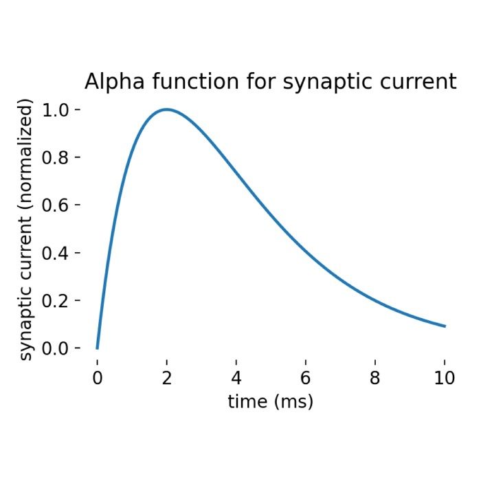
\[\begin{align} V_\text{m}(t) &= V_{\text{reset}} \quad\text{for}\quad t^* \leq t < t^* + t_{\text{ref}}. \end{align}\]

The synaptic current $I_{\text{syn}}(t)$ is modeled as an alpha function:

\[\begin{align} I_{\text{syn}}(t) &= I_{\text{syn, ex}}(t) + I_{\text{syn, in}}(t) \end{align}\]

where

\[\begin{align} I_{\text{syn, X}}(t) &= \sum_{j} w_j \sum_k i_{\text{syn, X}}(t-t_j^k-d_j) \end{align}\]

and $X \in { \text{ex}, \text{in} }$, i.e., either excitatory or inhibitory presynaptic neurons. $w_j$ is the synaptic weight, $t_j$ is the spike time of the presynaptic neuron, and $d_j$ is the axonal delay. $i_{\text{syn, X}}(t)$ controls individual post-synaptic currents (PSCs) and is defined as:

\[\begin{align} i_{\text{syn, X}}(t) &= \frac{t}{\tau_{\text{syn, X}}} e^{1 - \frac{t}{\tau_{\text{syn, X}}}} \Theta(t) \end{align}\]

where $\Theta(t)$ is the Heaviside step function and $\tau_{\text{syn, X}}$ is the synaptic time constant. This function causes the synaptic current to rise and decay in an alpha-shaped manner (rapid rise to a peak value, followed by a slower exponential decay). The PSCs are normalized such that:

\[\begin{align} i_{\text{syn, X}}(t= \tau_{\text{syn, X}}) &= 1 \end{align}\]

The total charge $q$ transfer due to a single PSC depends on the synaptic time constant according to:

\[\begin{align} q &= \int_0^{\infty} i_{\text{syn, X}}(t) dt = e \tau_{\text{syn, X}}. \end{align}\]

In our model, the external input $I_{\text{ext}}(t)$ will consist of a constant bias current and an alternating current (AC) generator to drive oscillations:

\[\begin{align} I_{\text{ext}}(t) &= I_{\text{bias}} + I_{\text{AC}}(t) \end{align}\]

with:

\[\begin{align} I_{\text{AC}}(t) &= A \sin(2 \pi f t) \end{align}\]

where:

$I_{\text{bias}}$ is the constant bias current.
$A$ is the amplitude of the AC generator.
$f$ is the frequency of the AC generator.

Oscillations in the input currents are crucial for synchronizing neuronal activity and enhancing spike-timing precision. They reflect the natural oscillatory dynamics observed in the olfactory bulb, helping to simulate realistic neural processing and facilitating the segregation and integration of information.

In addition to the deterministic inputs, a noise generator is included to simulate synaptic noise:

\[\begin{align} I_{\text{noise}}(t) &\sim \mathcal{N}(\mu, \sigma^2) \end{align}\]

where:

$\mu$ is the mean of the noise.
$\sigma$ is the standard deviation of the noise.

By including these elements in our model, we can more accurately represent the complex dynamics of the olfactory system and explore the principles of spike-timing-based computation.

Simulation code and results

The according simulation code is adapted and slightly modified from the NEST tutorial “Spike synchronization through subthreshold oscillation”ꜛ.

We begin by importing the necessary libraries:

import os
import matplotlib.pyplot as plt
import matplotlib.gridspec as gridspec
import numpy as np
import nest

# set global matplotlib properties for all plots:
plt.rcParams.update({'font.size': 12})
plt.rcParams["axes.spines.top"]    = False
plt.rcParams["axes.spines.bottom"] = False
plt.rcParams["axes.spines.left"]   = False
plt.rcParams["axes.spines.right"]  = False

nest.set_verbosity("M_WARNING")
nest.ResetKernel()

We create a network of 1000 neurons modeled with NEST’s iaf_psc_alphaꜛ neuron model implementation:

N = 1000  # number of neurons
bias_begin = 140.0  # minimal value for the bias current injection [pA]
bias_end   = 200.0  # maximal value for the bias current injection [pA]
T = 600  # simulation time (ms)

Next, we set the parameters for the input currents. We set up an alternating current generator (ac_generator) to drive oscillations in the input currents (35 Hz) with an amplitude of 50 pA. Additionally, we include a noise generator (noise_generator) to simulate synaptic noise with a standard deviation of 25 (mean is set to 0):

# parameters for the alternating-current generator
driveparams = {"amplitude": 50.0, "frequency": 35.0}
# parameters for the noise generator
noiseparams = {"mean": 0.0, "std": 25.0}
neuronparams = {
    "tau_m": 20.0,  # membrane time constant
    "V_th":  20.0,  # threshold potential
    "E_L":   10.0,  # membrane resting potential
    "t_ref":  2.0,  # refractory period
    "V_reset":0.0,  # reset potential
    "C_m":  200.0,  # membrane capacitance
    "V_m":    0.0,  # initial membrane potential
}

Now we create the corresponding simulation nodes. The neurons will receive a bias current that varies linearly from 140 pA (bias_begin) to 200 pA (bias_end) across the population. We also create a multimeter to record the membrane potential of the neurons:

neurons = nest.Create("iaf_psc_alpha", N)
spikerecorder = nest.Create("spike_recorder")
noise = nest.Create("noise_generator")
drive = nest.Create("ac_generator")
multimeter = nest.Create("multimeter", params={"record_from": ["V_m"]})

drive.set(driveparams)
noise.set(noiseparams)

neurons.set(neuronparams)
neurons.I_e = [(n * (bias_end - bias_begin) / N + bias_begin) for n in range(1, len(neurons) + 1)]

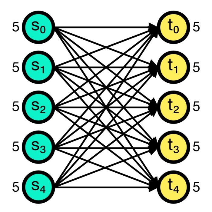
Next, we connect the nodes with each other, using the default all-to-all connection rule:

nest.Connect(drive, neurons)
nest.Connect(noise, neurons)
nest.Connect(neurons, spikerecorder)
nest.Connect(multimeter, neurons)

Finally, we simulate the network for T=600 ms:

nest.Simulate(T)

For further analysis, we extract the spike times and neuron IDs from the spike recorder for plotting:

# extract spike times and neuron IDs from the spike recorder for plotting:
spike_events = nest.GetStatus(spikerecorder, "events")[0]
spike_times = spike_events["times"]
neuron_ids = spike_events["senders"]

# combine the spike times and neuron IDs into a single array and sort by time:
spike_data = np.vstack((spike_times, neuron_ids)).T
spike_data_sorted = spike_data[spike_data[:, 0].argsort()]

# extract sorted spike times and neuron IDs:
sorted_spike_times = spike_data_sorted[:, 0]
sorted_neuron_ids = spike_data_sorted[:, 1]

# extract recorded data from the multimeter:
multimeter_events = nest.GetStatus(multimeter, "events")[0]

And the corresponding plot commands are as follows:

# spike raster plot and histogram of spiking rate:
fig = plt.figure(figsize=(6, 6))
gs = gridspec.GridSpec(5, 1)

# create the first subplot (3/4 of the figure)
ax1 = plt.subplot(gs[0:4, :])
ax1.scatter(sorted_spike_times, sorted_neuron_ids, s=9.0, color='mediumaquamarine', alpha=1.0)
ax1.set_title("spike synchronization through subthreshold oscillation:\nspike times (top) and rate (bottom)")
#ax1.set_xlabel("time [ms]")
ax1.set_xticks([])
ax1.set_ylabel("neuron ID")
ax1.set_xlim([0, T])
ax1.set_ylim([0, N])
ax1.set_yticks(np.arange(0, N+1, 100))

# create the second subplot (1/4 of the figure)
ax2 = plt.subplot(gs[4, :])
hist_binwidth = 5.0
t_bins = np.arange(np.amin(sorted_spike_times), np.amax(sorted_spike_times), hist_binwidth)
n, bins = np.histogram(sorted_spike_times, bins=t_bins)
heights = 1000 * n / (hist_binwidth * (N))
ax2.bar(t_bins[:-1], heights, width=hist_binwidth, color='violet')
#ax2.set_title(f"histogram of spiking rate vs. time")
ax2.set_ylabel("firing rate\n[Hz]")
ax2.set_xlabel("time [ms]")
ax2.set_xlim([0, T])

plt.tight_layout()
plt.show()

# plot the membrane potential and synaptic currents for 3 exemplary neurons:
fig = plt.figure(figsize=(6, 2))
sender = 100
idc_sender = multimeter_events["senders"] == sender
plt.plot(multimeter_events["times"][idc_sender], multimeter_events["V_m"][idc_sender], 
         label=f"neuron ID {sender}: ", alpha=1.0, c="k", lw=1.75, zorder=3)
sender = 200
idc_sender = multimeter_events["senders"] == sender
plt.plot(multimeter_events["times"][idc_sender], multimeter_events["V_m"][idc_sender], 
         label=f"neuron ID {sender}: ", alpha=0.8)
sender = 800
idc_sender = multimeter_events["senders"] == sender
plt.plot(multimeter_events["times"][idc_sender], multimeter_events["V_m"][idc_sender], 
         label=f"neuron ID {sender}: ", alpha=0.8)
plt.ylabel("membrane\npotential\n[mV]")
plt.xlabel("time [ms]")
plt.tight_layout()
plt.legend(loc="lower right")
plt.show()

Here is the resulting spike raster plot and histogram of the spiking rate:

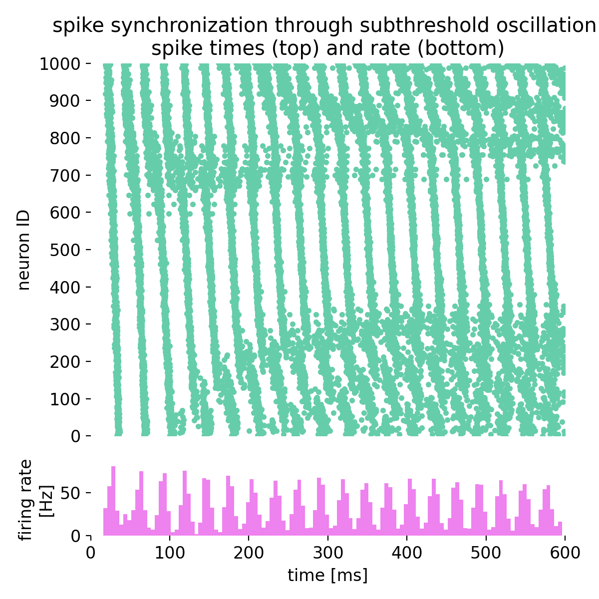Spike times (top) and spike frequency (bottom) of the network (1000 neurons). The spike raster plot shows the spike times of individual neurons over time, while the histogram displays the spiking rate as a function of time. The alternating current generator drives oscillations in the input currents, leading to synchronized spiking activity in the network. The noise generator introduces synaptic noise, adding variability to the spiking patterns. The network exhibits complex dynamics that can be further analyzed to understand the principles of spike-timing-based computation.

Let’s take a closer look at three exemplary neurons and their membrane potential traces:

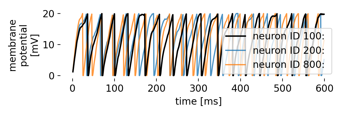Membrane potential traces of three exemplary neurons in the network. The membrane potential of each neuron exhibits distinct patterns of depolarization and repolarization, reflecting the underlying dynamics of the network.

The three traces, each from different regimes of the bias current, indeed show oscillatory behavior. However, while the oscillatory behavior remains evident throughout the simulated time course, synchronicity between the neurons is not always maintained. For some periods, the neurons spike synchronously, while at other times, the spike frequencies begins to diverge. This is due to the interplay between the alternating current generator, the noise generator, and the synaptic currents, which collectively shape the network’s activity. We can further examine this behavior on a more global scale by averaging the membrane potential traces of different groups of neurons, covering different regimes of the bias current, to identify common patterns and deviations:

# loop over all senders and collect all senders' V_m traces in a 2D array:
V_m_traces = np.zeros((N, T-1))
for sender_i, sender in enumerate(set(multimeter_events["senders"])):
    idc_sender = multimeter_events["senders"] == sender
    curr_V_m_trace = multimeter_events["times"][idc_sender]
    V_m_traces[sender_i, :] = multimeter_events["V_m"][idc_sender]

# plot neuron averages and std of membrane potential for different groups of neurons:
fig, ax = plt.subplots(5, 1, sharex=True, figsize=(6, 8), gridspec_kw={"hspace": 0.3})
axes = ax.flat
for i, (start, end) in enumerate([(800, 1000), (600, 800), (400, 600), (200, 400),(0, 200) ]):
    V_m_mean = np.mean(V_m_traces[start:end, :], axis=0)
    V_m_std = np.std(V_m_traces[start:end, :], axis=0)
    axes[i].plot(multimeter_events["times"][idc_sender], V_m_mean, label="mean membrane potential", c="k")
    axes[i].fill_between(multimeter_events["times"][idc_sender], V_m_mean - V_m_std, V_m_mean + V_m_std, color='gray', alpha=0.5)
    axes[i].set_ylabel(f"membrane\npotential $V_m$\n[mV]")
    axes[i].set_title(f"average and std of neurons {start} to {end}")
axes[-1].set_xlabel("time [ms]")
plt.tight_layout()
plt.show()

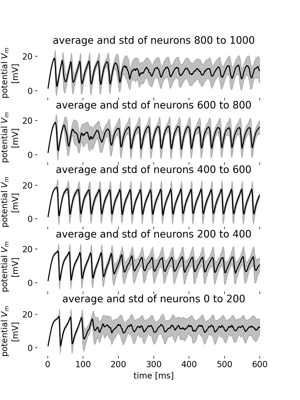Average membrane potential trace and standard deviations for different groups of neurons.

From the average membrane potential traces of the different groups of neurons, we can observe that the synchronicity within a group is almost maintained at the beginning of the simulation (low standard deviation). However, as the simulation progresses, the synchronicity within almost all groups starts to break as the standard deviation of the membrane potential increases. This is not true for the group of neurons with IDs 400-600, where synchronicity, frequency, and amplitude of the oscillations remain almost constant. The groups of neurons with IDs 800-1000 and IDs 0 to 200 show the highest standard deviation with decreasing amplitude of the oscillations over the course of the simulation. An interesting behavior is observed for the group of neurons with IDs 600-800, where both the standard deviation increase (and thus the synchronicity decreases) and the amplitude of the oscillations increases for just a short period of time shortly after the beginning of the simulation. The different behavior across the groups of neurons reflects the complex and variable dynamics of the network as already observed in the spike raster plot.

You can further investigate the network dynamics by modifying the parameters of the alternating current generator, the noise generator, and the synaptic currents. By exploring different input patterns and noise levels, you can observe how these factors influence the synchronization and spiking activity of the network. This will provide valuable insights into the principles of spike-timing-based computation and the role of oscillatory inputs and synaptic noise in shaping neural activity.

Conclusion

In this tutorial, we have explored the principles of spike-timing-based computation in the context of olfactory processing using a simple network model proposed by Brody and Hopfieldꜛ. By simulating a network of spiking neurons with NEST, we have demonstrated how oscillatory input currents, synaptic noise, and alpha-shaped postsynaptic currents can shape the dynamics of the network and influence spike synchronization. The resulting spike raster plot and membrane potential traces provide insights into the complex interactions between neurons and the emergence of synchronized spiking activity. By analyzing the average membrane potential traces of different groups of neurons, we have observed how synchronicity within the network evolves over time, highlighting the importance of oscillatory inputs and synaptic noise in shaping neural activity.

This tutorial serves as a starting point for exploring spike-timing-based computation and its applications in neural processing. By modifying the parameters of the network model and exploring different input patterns, you can further investigate the dynamics of the network and gain a deeper understanding of how spiking neurons encode and process information.

The complete code used in this blog post is available in this Github repositoryꜛ (spike_synchronization_through_oscillation.py). Feel free to modify and expand upon it, and share your insights.