Frequency-current (f-I) curves

In this short tutorial, we will explore the concept of frequency-current (f-I) curves exemplified by the Hodgkin-Huxley neuron model. The f-I curve describes the relationship between the input current to a neuron and its firing rate. We will use the NEST simulator to simulate the behavior of a single Hodgkin-Huxley neuron and plot its f-I curve.

f-I curves

The f-I curve or frequency-current curve is a fundamental concept in neuroscience that describes the relationship between the input current to a neuron and the firing rate (frequency) of that neuron. It is a graphical representation used to understand how a neuron’s output firing rate varies with changes in the input current.

The key concepts of generating a f-I curve is a as follows:

1. Input Current (I): This is the external current injected into the neuron, often referred to as the “stimulus current” or “input current.” It is typically measured in picoamperes (pA) or nanoamperes (nA).
2. Firing Rate (f): This is the neuron’s output in response to the input current, measured in spikes per second (Hz). It represents how frequently a neuron fires action potentials.

The shape of the f-I curve can provide insights into the neuron’s response properties. Here are some common characteristics:

• threshold: The minimum input current required to elicit action potentials. Below this threshold, the neuron does not fire.
• saturation: At very high input currents, the firing rate may plateau, indicating that the neuron has reached its maximum firing capacity.
• slope: The steepness of the f-I curve indicates how sensitive the neuron is to changes in input current. A steep slope means small changes in input current cause large changes in firing rate.

Types of f-I curves

Different types of neurons exhibit different f-I curves based on their intrinsic properties and the input they receive. Here are some common types:

• Linear f-I Curve: Some neurons have a relatively linear relationship between input current and firing rate. This means that as the input current increases, the firing rate increases proportionally.
• Non-linear f-I Curve: Many neurons exhibit a non-linear f-I curve, where the relationship between input current and firing rate is not proportional. This can include sigmoidal shapes, showing a more complex relationship with thresholds and saturation points.
• Threshold-linear f-I Curve: A combination where the curve is linear above a certain threshold current but zero below it.

Importance of the f-I curve

The f-I curve serves multiple essential functions in both experimental and computational contexts. It provides insights into how neurons translate input currents into output firing rates, thereby playing a key role in understanding neural coding and information processing in the brain.

Characterizing neuronal response

The f-I curve helps in understanding how neurons encode information. By examining the relationship between input current and firing rate, one can infer how different stimuli are represented by neuronal activity. This is fundamental to deciphering the brain’s ‘language’ of spikes and how sensory inputs are processed and perceived.

Different neurons have different f-I curves, reflecting their unique response properties. For example, some neurons might be highly sensitive to small changes in input current, while others may require larger currents to change their firing rates significantly. By characterizing these properties, one can categorize neurons into functional types and understand their roles in neural circuits.

The f-I curve also reveals important aspects such as the threshold current required to elicit firing and the saturation point where further increases in input current no longer increase the firing rate. These features help in understanding the operating range of neurons and their potential role in processing various intensity levels of stimuli.

Computational modeling

In computational neuroscience, the f-I curve is used to develop and refine neuron models. Accurate f-I curves ensure that simulated neurons behave similarly to biological neurons, which is crucial for realistic neural network models. This helps in studying complex neural dynamics and testing hypotheses about brain function.

The f-I curve allows for fine-tuning model parameters to match experimental data. Parameters such as membrane conductance, capacitance, and synaptic weights can be adjusted to ensure that the model’s f-I curve aligns with that of real neurons, thereby enhancing the model’s validity.

Models incorporating accurate f-I curves can predict how neurons will respond to novel stimuli. This predictive capability is valuable for understanding brain function, designing neural prosthetics, and developing treatments for neurological disorders.

Experimental studies

Experimentally, f-I curves are used to classify different types of neurons. For example, excitatory and inhibitory neurons often have distinct f-I curves, reflecting their different roles in neural circuits. By analyzing these curves, one can identify neuron types and understand their contributions to brain function.

The shape and parameters of the f-I curve can also indicate the health of neurons. Changes in the f-I curve can signal pathological conditions such as neurodegenerative diseases or the effects of drugs. Monitoring these changes helps in diagnosing and understanding the progression of neurological disorders.

Simulating the f-I curve of a Hodgkin-Huxley neuron

Here’s a simple Python example using the NEST simulator to calculate the f-I curve of a Hodgkin-Huxley neuron. The code simulates a range of input currents and records the firing rate of the neuron in response to each current level. The resulting plot shows the f-I curve of the neuron. The code is adapted from the NEST tutorial “Example using Hodgkin-Huxley neuron”ꜛ

import os
import matplotlib.pyplot as plt
import matplotlib.gridspec as gridspec
import numpy as np
import nest
import nest.raster_plot

# set global properties for all plots:
plt.rcParams.update({'font.size': 12})
plt.rcParams["axes.spines.top"]    = False
plt.rcParams["axes.spines.bottom"] = False
plt.rcParams["axes.spines.left"]   = False
plt.rcParams["axes.spines.right"]  = False

nest.set_verbosity("M_WARNING")
nest.ResetKernel()

# define simulation time:
time = 1000

# amplitude range (in pA):
I_start = 0
I_stopt = 2000
I_step  = 20

# define simulation step size (in mS):
h = 0.1

# create a Hodgkin-Huxley neuron and a spikerecorder node:
neuron = nest.Create("hh_psc_alpha")
spikerecorder = nest.Create("spike_recorder")
spikerecorder.record_to = "memory"

nest.Connect(neuron, spikerecorder, syn_spec={"weight": 1.0, "delay": h})

# simulation loop:
n_data = int(I_stopt / float(I_step))
amplitudes  = np.zeros(n_data)
event_freqs = np.zeros(n_data)
for i, amp in enumerate(range(I_start, I_stopt, I_step)):
    neuron.I_e = float(amp)
    
    nest.Simulate(1000)         # one second warm-up time for equilibrium state
    spikerecorder.n_events = 0  # then reset spike counts
    nest.Simulate(time)         # another simulation call to record firing rate

    n_events = spikerecorder.n_events
    amplitudes[i]  = amp
    event_freqs[i] = n_events / (time / 1000.0)
    print(f"Simulating with current I={amp} pA -> {n_events} spikes in {time} ms ({event_freqs[i]} Hz)")

# plot the results:
plt.figure(figsize=(5, 4))
plt.plot(amplitudes, event_freqs, lw=2.0)
plt.xlabel("input current (pA)")
plt.ylabel("firing rate (Hz)")
plt.title("Firing rate vs. input current\nof a Hodgkin-Huxley neuron")
plt.tight_layout()
plt.grid(True)
plt.show()

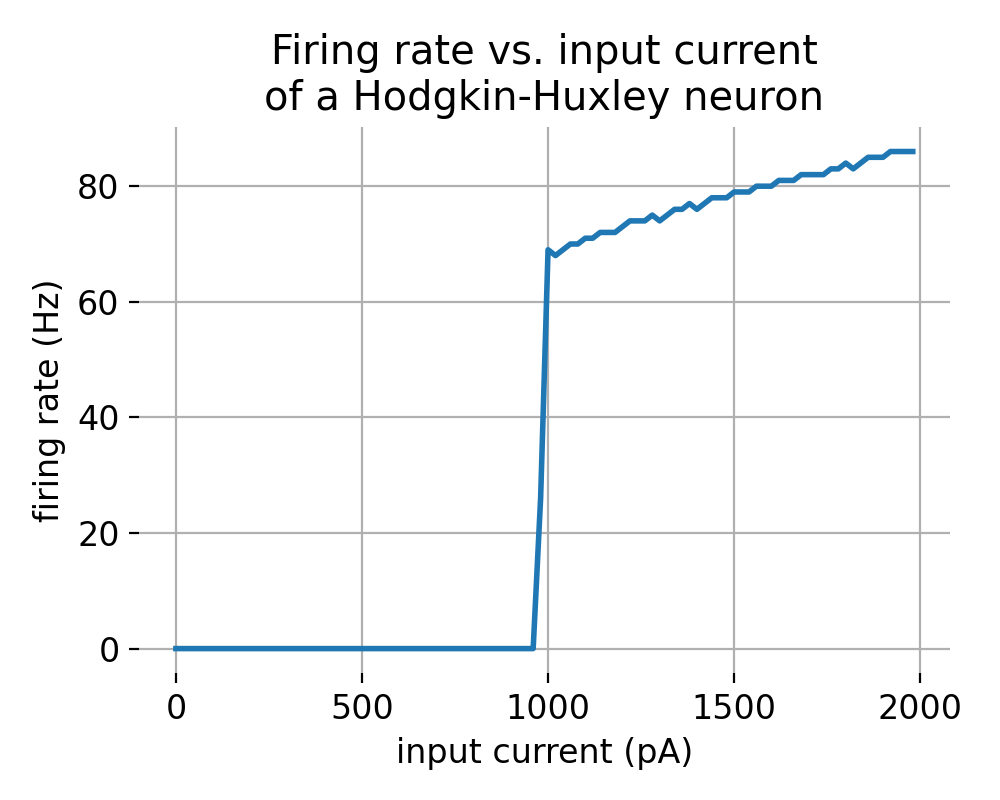
f-I curve of a Hodgkin-Huxley neuron simulated using the NEST simulator. The plot shows the firing rate of the neuron in response to varying input currents. The curve exhibits a threshold, a linear region, and a saturation point, typical of many neuron types.

Conclusion

The f-I curve is a crucial tool in neuroscience for understanding the relationship between a neuron’s input and its output. It provides valuable insights into neuronal behavior, response characteristics, and is fundamental in both experimental and computational neuroscience.

The complete code used in this blog post is available in this Github repositoryꜛ (fi_curve.py). Feel free to modify and expand upon it, and share your insights.

References and useful links

• Wikipedia article on “f-I curve”ꜛ
• B. Ermentrout, Linearization of F-I curves by adaptation, 1998, Neural Computation. 10 (7): 1721–1729, doi: 10.1162/089976698300017106ꜛ
• A. L. Hodgkin, The local electric changes associated with repetitive action in a non-medullated axon, 1948, The Journal of physiology, doi: 10.1113/jphysiol.1948.sp004260ꜛ
• Neuromatch’s “Tutorial 1: Neural Rate Models”ꜛ
• NEST’s tutorial “Example using Hodgkin-Huxley neuron”ꜛ
• NEST’s hh_psc_alpha model descriptionꜛ