Oscillatory population dynamics of GIF neurons simulated with NEST

In this tutorial, we will explore the oscillatory population dynamics of generalized integrate-and-fire (GIF) neurons simulated with NEST. The GIF neuron model is a biophysically detailed model that captures the essential features of spiking neurons, including spike-frequency adaptation and dynamic threshold behavior. By simulating such a population of neurons, we can observe how these neurons interact and generate oscillatory firing patterns.

Mathematical formulation

NEST’s implementation of the current-based generalized integrate-and-fire (GIF) neuron modelꜛ with exponential postsynaptic currents (PSCs) is based on the model proposed by Mensi et al. (2012)ꜛ and Pozzorini et al. (2015)ꜛ. This model features both an adaptation current and a dynamic threshold for spike-frequency adaptation.

Membrane potential dynamics

The membrane potential $V(t)$ of the GIF neuron model is described by the following differential equation:

\[\begin{align*} C \cdot {dV(t) \over dt} =& -g_L \cdot (V(t)-E_L) - \eta_1(t) \\ &- \eta_2(t) - \ldots - \eta_n(t) + I(t) \end{align*}\]

where $C$ is the membrane capacitance, $V(t)$ is the membrane potential, $g_L$ is the leak conductance, $E_L$ is the leak reversal potential, $\eta_i(t)$ are the adaptation or spike-triggered currents (stc), and $I(t)$ is the input current.

Adaptation currents

The adaptation currents $\eta_i(t)$ are described by the following differential equations:

\[\tau_\eta{_i} \cdot \frac{d{\eta_i}}{dt} = -\eta_i\]

Upon the occurrence of a spike, these currents are incremented by a fixed amount $q_{\eta_i}$:

\[\eta_i = \eta_i + q_{\eta_i}\]

Firing intensity and dynamic threshold

Spikes are produced stochastically according to a point process with the firing intensity:

\[\lambda(t) = \frac{\lambda_0}{\Delta_V} e^{(V(t)-V_T(t))}\]

where $V_T(t)$ is the dynamic, time-dependent firing threshold, $\lambda_0$ is the firing intensity at threshold, and $\Delta_V$ is the slope factor. The dynamic threshold is defined as:

\[\begin{align*} V_T(t) =& V_{T_{star}} + \gamma_1(t) + \gamma_2(t) + \ldots + \gamma_m(t) \\ =& V_{T_{star}} + \sum_{j} \gamma_j(t) \end{align*}\]

where $\gamma_i(t)$ is a kernel of spike-triggered currents (stc) for the dynamic threshold. The neuron can have an arbitrary number of them. Its dynamics are described by the following differential equations:

\[\tau_{\gamma_i} \cdot {d\gamma_i \over dt} = -\gamma_i\]

Similarly, upon a spike, each dynamic threshold current $\gamma_j(t)$ is updated by $q_{\gamma_j}$:

\[\gamma_i = \gamma_i + q_{\gamma_i}\]

Oscillatory behavior

The described GIF neuron tends to show oscillatory behavior due to the dynamic interplay between spike-frequency adaptation currents and the dynamic firing threshold.

The adaptation currents $\eta_i(t)$ act to modulate the neuron’s excitability over time. After each spike, $\eta_i(t)$ increases by $q_{\eta_i}$, which causes a temporary reduction in the membrane potential $V(t)$, making it less likely for the neuron to fire immediately again. These currents decay exponentially with time constants $\tau_{\eta_i}$. If the neuron continues to receive input, these adaptation currents lead to a rhythmic pattern of firing and resting, as they counterbalance the input current $I(t)$.

The dynamic threshold $V_T(t)$ introduces another layer of temporal modulation. After a spike, $\gamma_j(t)$ increases by $q_{\gamma_j}$, raising the threshold $V_T(t)$ and making it harder for subsequent spikes to occur immediately. This also decays exponentially with a time constant $\tau_{\gamma_j}$. The interaction between the rising and falling $V_T(t)$ due to spike-triggered changes creates a pattern where the neuron alternates between being highly excitable and less excitable.

The combination of spike-frequency adaptation through $\eta_i(t)$ and the dynamic threshold through $\gamma_j(t)$ leads to oscillations. After a spike, both $\eta_i(t)$ and $\gamma_j(t)$ increase, causing a temporary decrease in the likelihood of firing. As these factors decay, the membrane potential $V(t)$ gradually approaches the baseline level until the input current $I(t)$ is sufficient to trigger another spike. This cycle of spike-triggered adaptation and recovery results in oscillatory firing patterns.

The timescale of these oscillations is determined by the time constants $\tau_{\eta_i}$ and $\tau_{\gamma_j}$. Typically, these time constants are on the order of tens to hundreds of milliseconds, matching the frequency range of observed neuronal oscillations in the brain (e.g., theta, alpha, and beta rhythms).

Adjustable model parameters in NEST

The NEST implementation of the GIF neuron model with exponential PSCs accepts the following parameters:

Membrane parameters	Unit	Description
C_m	pF	Membrane capacitance
t_ref	ms	Refractory period
V_reset	mV	Reset potential
E_L	mV	Leak reversal potential
g_L	nS	Leak conductance
I_e	pA	constant external input current

Spike adaptation and firing intensity parameters	Unit	Description
q_stc	list of nA	Values added to spike-triggered currents (stc) after each spike emission
tau_stc	list of ms	Time constants of spike-triggered currents (stc)
q_sfa	list of mV	Values added to spike-frequency adaptation (sfa) after each spike emission
tau_sfa	list of ms	Time constants of spike-frequency adaptation (sfa)
Delta_V	mV	Slope factor or stochasticity level of the firing intensity function
lambda_0	Hz	Stochastic intensity at firing threshold V_T
V_T_star	mV	Baseline of the dynamic threshold V_T

Synaptic parameters	Unit	Description
tau_syn_ex	ms	Time constant of the excitatory synaptic current
tau_syn_in	ms	Time constant of the inhibitory synaptic current

Simulation with NEST

We create a population of 100 GIF neurons using the gif_psc_expꜛ model implemented in NEST with a connection probability of 0.3 and synaptic weights of 30 pA. Further model parameters are chosen according Pozzorini et al. (2015)ꜛ. We will also add a Poisson noise input to the population to drive the oscillatory dynamics. The simulation will run for 2000 ms, and we will record the spike times and neuron IDs for plotting. The according simulation code is adapted and slightly modified from the NEST tutorial “Population of GIF neuron model with oscillatory behavior”ꜛ.

Let’s start by importing the necessary libraries and defining the model parameters:

import matplotlib.pyplot as plt
import matplotlib.gridspec as gridspec
import numpy as np
import nest
import nest.raster_plot

nest.set_verbosity("M_WARNING")
nest.ResetKernel()

dt = 0.1 # simulation resolution [ms]
T = 2000.0 # simulation time [ms]

# set the resolution of the simulation:
nest.resolution = dt

# define the parameters of the GIF neuron model:
neuron_params = {
    "C_m": 83.1,
    "g_L": 3.7,
    "E_L": -67.0,
    "Delta_V": 1.4,
    "V_T_star": -39.6,
    "t_ref": 4.0,
    "V_reset": -36.7,
    "lambda_0": 1.0,
    "q_stc": [56.7, -6.9],
    "tau_stc": [57.8, 218.2],
    "q_sfa": [11.7, 1.8],
    "tau_sfa": [53.8, 640.0],
    "tau_syn_ex": 10.0,
}

# define the parameters of the population and noise:
N_ex = 100  # size of the population
p_ex = 0.3  # connection probability inside the population
w_ex = 30.0  # synaptic weights inside the population (pA)

N_noise    = 67  # size of Poisson group, default: 50
rate_noise = 12.0  # firing rate of Poisson neurons (Hz), default: 12
w_noise    = 20.0  # synaptic weights from Poisson to population neurons (pA)

Next, we create the nodes, establish connections, and run the simulation:

# create nodes:
population = nest.Create("gif_psc_exp", N_ex, params=neuron_params)
noise = nest.Create("poisson_generator", N_noise, params={"rate": rate_noise})
spikerecorder = nest.Create("spike_recorder")

# establish connections:
nest.Connect(population, population, {"rule": "pairwise_bernoulli", "p": p_ex}, syn_spec={"weight": w_ex})
nest.Connect(noise, population, "all_to_all", syn_spec={"weight": w_noise})
nest.Connect(population, spikerecorder)

nest.Simulate(T)

Finally, we extract the spike times and neuron IDs for plotting the raster plot and the firing rate histogram:

# extract spike times and neuron IDs for plots:
spike_events = nest.GetStatus(spikerecorder, "events")[0]
spike_times = spike_events["times"]
neuron_ids = spike_events["senders"]

# combine the spike times and neuron IDs into a single array and sort by time:
spike_data = np.vstack((spike_times, neuron_ids)).T
spike_data_sorted = spike_data[spike_data[:, 0].argsort()]

# extract sorted spike times and neuron IDs:
sorted_spike_times = spike_data_sorted[:, 0]
sorted_neuron_ids = spike_data_sorted[:, 1]

Here are the corresponding plot commands:

fig = plt.figure(figsize=(6, 6))
gs = gridspec.GridSpec(5, 1)

ax1 = plt.subplot(gs[0:4, :])
ax1.scatter(sorted_spike_times, sorted_neuron_ids, s=9.0, color='mediumaquamarine', alpha=1.0)
ax1.set_title("Oscillatory population dynamics of GIF neurons:\nspike times (top) and rate (bottom)")
ax1.set_xticks([])
ax1.set_ylabel("neuron ID")
ax1.set_xlim([0, T])
ax1.set_ylim([0, N_ex])
ax1.spines["top"].set_visible(False)
ax1.spines["bottom"].set_visible(False)
ax1.spines["left"].set_visible(False)
ax1.spines["right"].set_visible(False)
ax1.set_yticks(np.arange(0, N_ex+1, 10))

ax2 = plt.subplot(gs[4, :])
hist_binwidth = 5.0
t_bins = np.arange(np.amin(sorted_spike_times), np.amax(sorted_spike_times), hist_binwidth)
n, bins = np.histogram(sorted_spike_times, bins=t_bins)
heights = 1000 * n / (hist_binwidth * (N_ex))
ax2.bar(t_bins[:-1], heights, width=hist_binwidth, color='violet')
ax2.spines["top"].set_visible(False)
ax2.spines["bottom"].set_visible(False)
ax2.spines["left"].set_visible(False)
ax2.spines["right"].set_visible(False)
ax2.set_ylabel("firing rate\n[Hz]")
ax2.set_xlabel("time [ms]")
ax2.set_xlim([0, T])

plt.show()

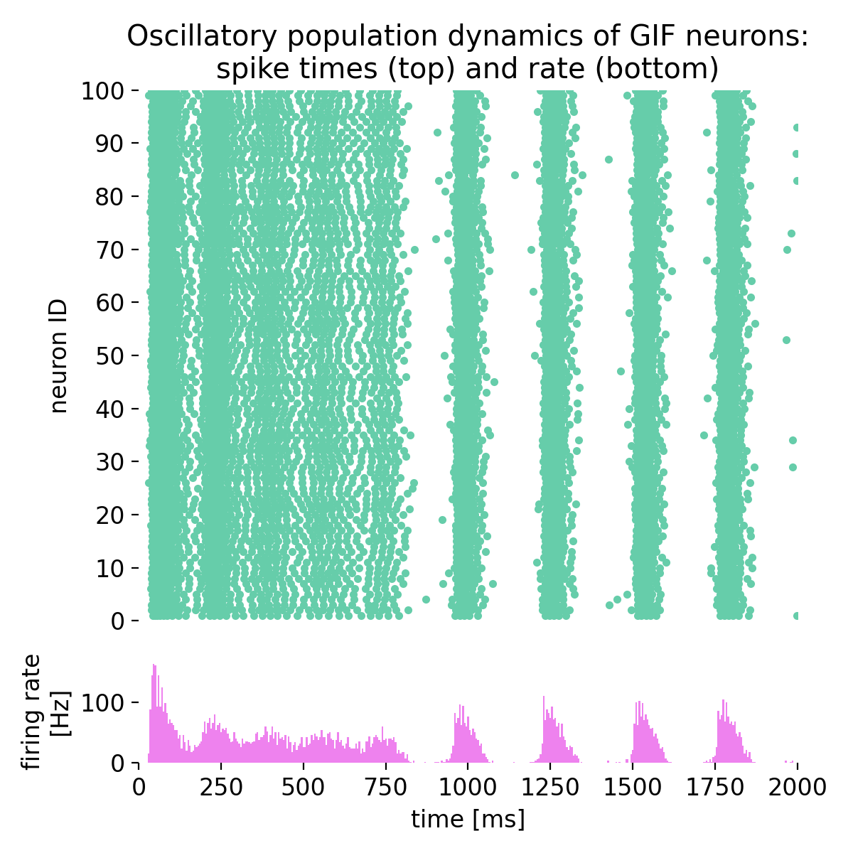Oscillatory population dynamics of GIF neurons: spike times (top) and spike frequency (bottom).

With the chosen parameters, the population of GIF neurons indeed exhibits oscillatory behavior, characterized by rhythmic firing patterns and alternating periods of high and low excitability. The interplay between spike-frequency adaptation and the dynamic threshold leads to the emergence of oscillations in the firing rate, as seen in the raster plot and the firing rate histogram.

The model is sensitive to the choice of parameters, such as the size of the Poisson noise group, the time constants of spike-triggered currents (stc; tau_stc), and the time constants of spike-frequency adaptation (sfa; tau_sfa). Adjusting these parameters can lead to different oscillatory patterns and firing rates, providing insights into the mechanisms underlying rhythmic neuronal activity in the brain:

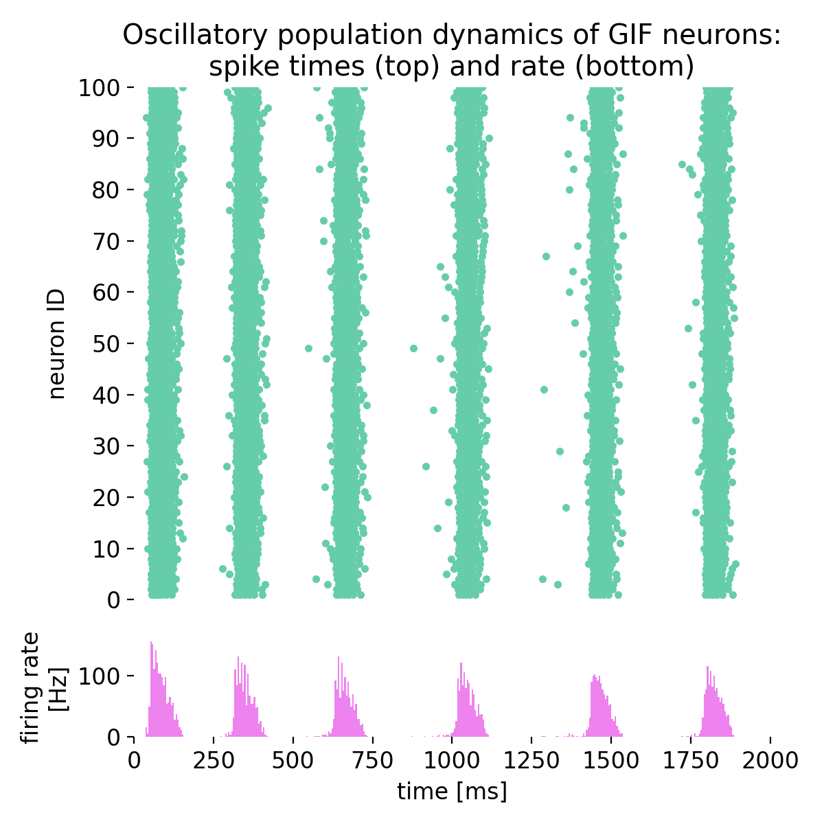Same simulation as before, but with a Poisson noise group of just 50 neurons (instead of 67).

Same simulation as before, but with different time constants of spike-triggered currents (stc; tau_stc): 47.8 ms and 218.2 ms instead of 57.8 ms and 218.2 ms.

Same simulation as before, but with different time constants of spike-frequency adaptation (sfa; tau_sfa): 73.8 ms and 640.0 ms instead of 53.8 ms and 640.0 ms.

Conclusion

The oscillatory dynamics of the GIF neuron model capture essential features of neuronal activity observed in the brain and provide insights into the mechanisms underlying rhythmic firing patterns in neural circuits. This example demonstrates, how we can use NEST for studying the population dynamics and exploring the effects of different model parameters. By adjusting the parameters of the model, we can simulate a wide range of firing patterns and investigate the role of, e.g., spike-frequency adaptation and dynamic thresholds in shaping neuronal activity. This approach can help us understand how neural circuits generate oscillations and how these oscillations contribute to information processing in the brain.

The complete code used in this blog post is available in this Github repositoryꜛ. Feel free to modify and expand upon it, and share your insights.

References and useful links

• NEST tutorial “Population of GIF neuron model with oscillatory behavior”ꜛ
• NEST’s gif_psc_exp model descriptionꜛ
• Mensi S, Naud R, Pozzorini C, Avermann M, Petersen CC, Gerstner W, Parameter extraction and classification of three cortical neuron types reveals two distinct adaptation mechanisms, 2012, Journal of Neurophysiology, 107(6):1756-1775. DOI: 10.1152/jn.00408.2011ꜛ
• Pozzorini C, Mensi S, Hagens O, Naud R, Koch C, Gerstner W, Automated high-throughput characterization of single neurons by means of simplified spiking models, 2015, PLoS Computational Biology, 11(6), e1004275. DOI: 10.1371/journal.pcbi.1004275