Connection concepts in NEST
In the previous post, we learned about the basic concepts of the NEST simulator and how to create a simple single neuron model. This time, we will take a closer look at the connection concepts in NEST, which are crucial for building more complex neural networks.
Introduction
Connectionsꜛ in NEST are created via the
nest.Connection(pre, post, conn_spec, syn_spec)
commandꜛ, where pre and post are the pre- and post-synaptic nodes (e.g., single neurons or neuron populations), respectively. The conn_spec and syn_spec arguments define the connection rule and the synapse model, respectively. If the latter two are omitted, the default all_to_all connection and the default static_synapseꜛ are used. The static synapse is a synapse, where the synaptic strength (or weight) does not evolve over time and remains at a defined constant value.
conn_spec expects a connection rule alongside additional rule-specific parameters (if any). The following connection rules are available:
all_to_all(default)one_to_onepairwise_bernoulli(parameter:p)symmetric_pairwise_bernoulli(parameter:p)pairwise_poisson(parameter:pairwise_avg_num_conns)fixed_indegree(parameter:indegree)fixed_outdegree(parameter:outdegree)fixed_total_number(parameter:N)
For instance, connection using the pairwise_bernoulli rule would look like this:
n = 5
m = 5
p = 0.5
S = nest.Create('iaf_psc_alpha', n)
T = nest.Create('iaf_psc_alpha', m)
conn_spec = {'rule': 'pairwise_bernoulli', 'p': p}
nest.Connect(S, T, conn_spec)
The chosen synapse model (syn_spec) along with its parameters such as the synaptic weight, delay, and model-specific parameters controls the strength of the connection between the pre- and post-synaptic neurons. The synaptic weight determines how strongly a spike from a presynaptic neuron affects the postsynaptic neuron. Thus, it quantifies the efficacy of the synapse in transmitting the signal. An exemplary syn_spec definition looks like this:
n = 10
neuron_dict = {'tau_syn': [0.3, 1.5]}
A = nest.Create('iaf_psc_exp_multisynapse', n, neuron_dict)
B = nest.Create('iaf_psc_exp_multisynapse', n, neuron_dict)
syn_spec_dict ={'synapse_model': 'static_synapse',
                'weight': 2.5,
                'delay': 0.5,
                'receptor_type': 1}
nest.Connect(A, B, syn_spec=syn_spec_dict)
Further details on synapse specification can be found in the NEST documentationꜛ.
In the following, we will discuss the different connection concepts in more detail. For consistency, we will call a single neuron a “node” and a collection of nodes a “node collection” (or just collection). Pre- and postsynaptic node collections are further referred to as $S$ and $T$ for the source and target node collections, respectively. A single connection between two nodes is called an edge, while a group of edges that connect groups of nodes with similar properties (i.e, populations) is called a projection. In these terms, the nest.Connection() function establishes a projection between the source and target node collection.
Connection rules
Autapses and multapses
The conn_spec argument can receive two additional parameters, autapses and multapses. Autapases are self-connections of a node and multapses are multiple connections between the same pair of nodes:
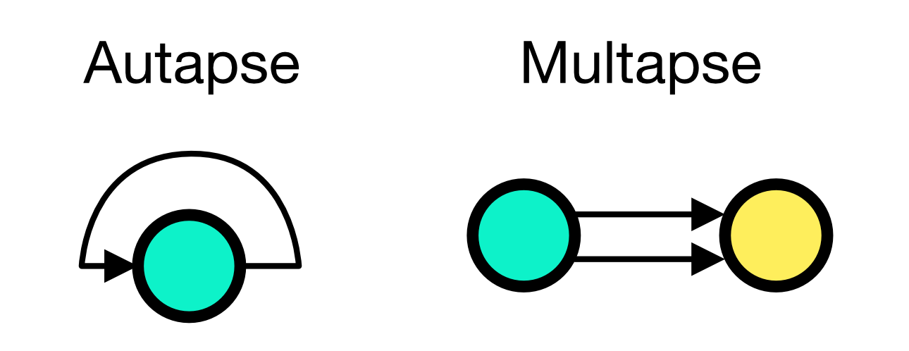
Autapses and multapses paradigms. If autapses is set to True (default), a neuron can connect to itself. If multapses is set to True (default), multiple connections between the same pair of nodes are allowed.
autapses and multapses are both set to True by default.
All to all
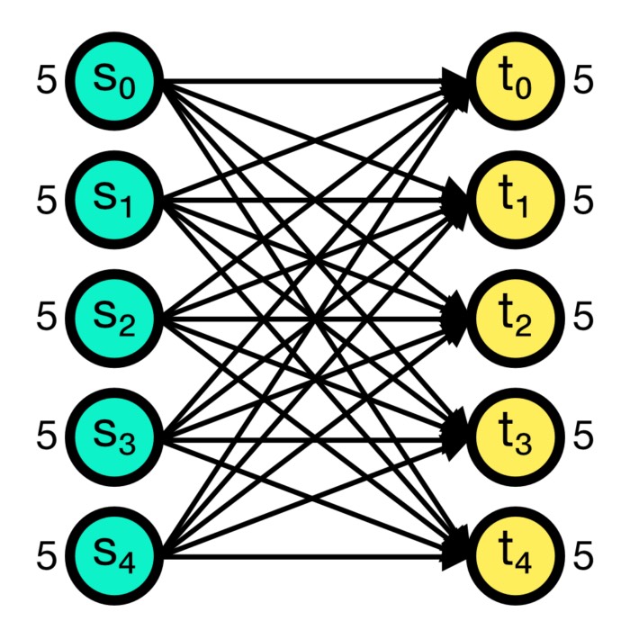
The all_to_all connection rule connects all pre-synaptic nodes (source) to all post-synaptic nodes (target). This is the default connection rule in NEST. The all_to_all rule does not require any additional parameters.
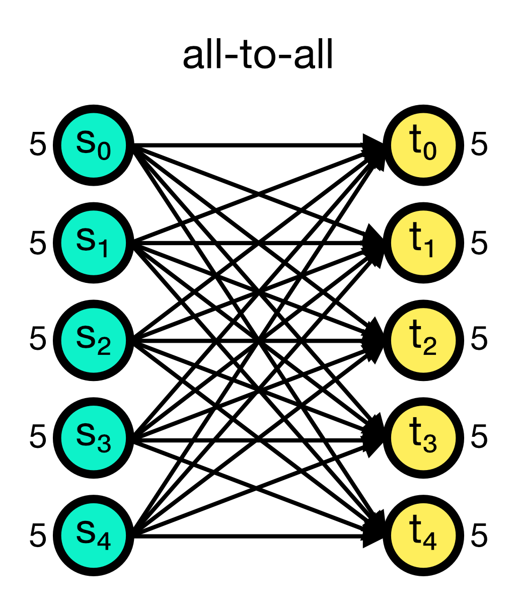
All-to-all connection scheme in NEST. All pre-synaptic nodes (source) are connected to all post-synaptic nodes (target). Numbers beside the nodes indicate the number of out- and in-connections, respectively.
Example:
n = 5
m = 5
S = nest.Create('iaf_psc_alpha', n)
T = nest.Create('iaf_psc_alpha', m)
nest.Connect(S, T, 'all_to_all')
nest.Connect(S, T)  # this is equivalent
To explicitly connect source and target nodes, the respective node IDs from the node collections must be extracted and then be connected using the one-to-one connection rule. For instance, in the following example we connect the 3rd, 4th, and 1st source nodes to the 8th, 6th, and 9th target nodes, respectively:
n = 5
m = 5
S = nest.Create('iaf_psc_alpha', n) # node ids: 1..5
T = nest.Create('iaf_psc_alpha', m) # node ids: 6..10
# source-target pairs: (3,8), (4,1), (1,9)
nest.Connect([3,4,1], [8,6,9], 'one_to_one')
One to one
The one_to_one connection rule connects each pre-synaptic node to exactly one post-synaptic node, i.e., the $i$-th source node in the source node collection $S$ is connected to the $i$-th target node in the target node collection $T$. The number of pre- and post-synaptic nodes must be equal. The one_to_one rule does not require any additional parameters.
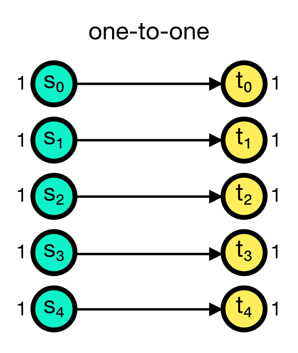
One-to-one connection scheme in NEST. Each pre-synaptic node is connected to exactly one post-synaptic node. he number of pre- and post-synaptic nodes must be equal.
Example:
n = 5
S = nest.Create('iaf_psc_alpha', n)
T = nest.Create('spike_recorder', n)
nest.Connect(S, T, 'one_to_one')
Deterministic connection rules: Both all_to_all and one_to_one are deterministic connection rules, i.e., precisely defined sets of connections are established between the source and target nodes without any randomness or variability across network realizations.
Probabilistic connection rules: In contrast, probabilistic connection rules such as pairwise_bernoulli or pairwise_poisson establish connections between the source and target nodes based on a probabilistic rule. This leads to variability in the network structure across different network realizations. However, such connectivity leads to specific expectation values of network characteristics, such as degree distributions or correlation structure.
Pairwise Bernoulli
The pairwise_bernoulli connection rule establishes connections between the source and target nodes based on a Bernoulli process. The probability p of establishing a connection between any pair of nodes is given as an additional parameter. The pairwise_bernoulli rule requires the parameter p to be set. Multapses cannot be established with this rule as each possible edge is visited only once, independent of setting allow_multapses to True.
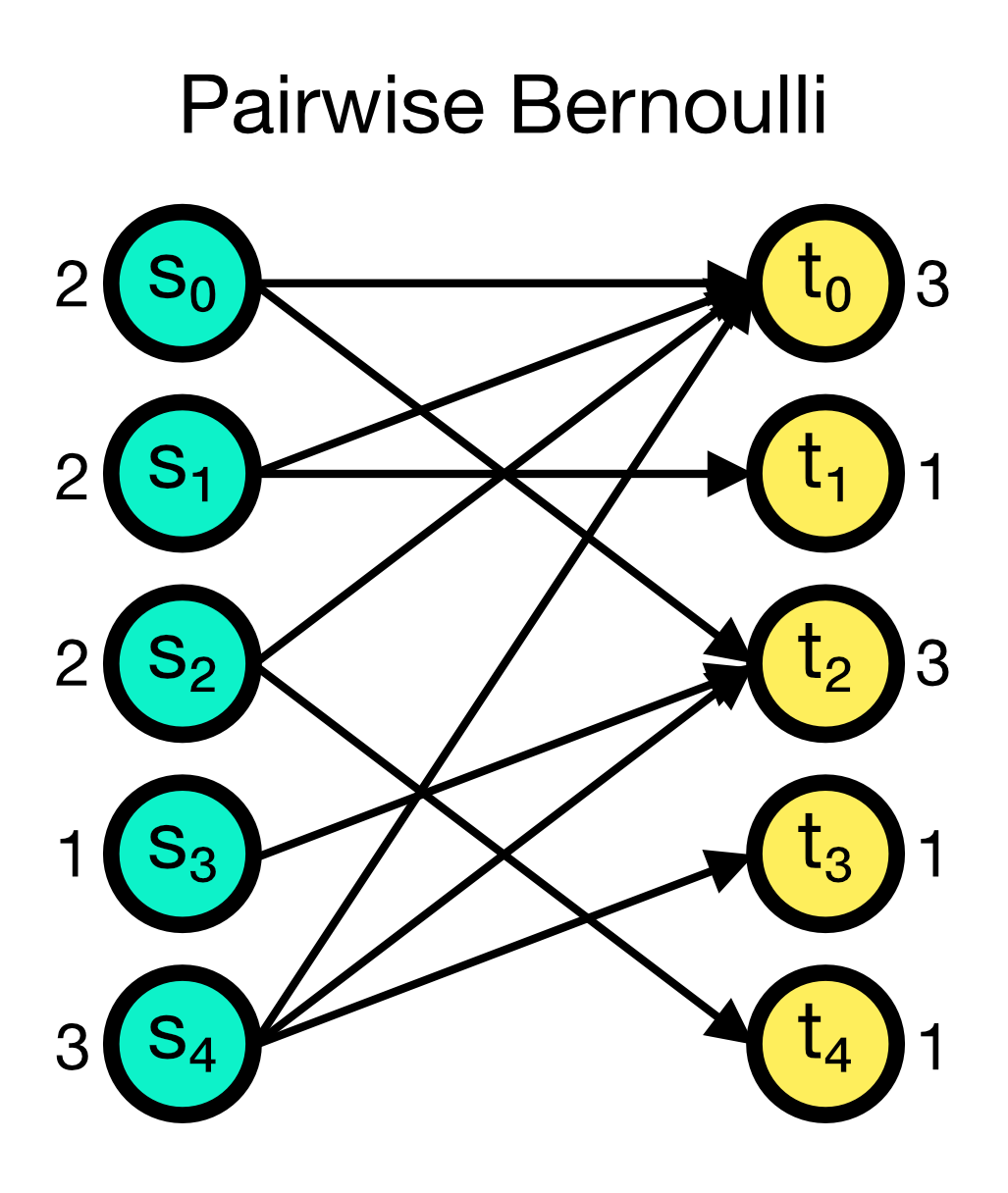
Pairwise Bernoulli connection scheme in NEST. Connections are established between the source and target nodes based on a Bernoulli process with probability $p$. Each possible edge is visited only once, independent of setting allow_multapses to True.
Example:
n = 5
m = 5
p = 0.5
S = nest.Create('iaf_psc_alpha', n)
T = nest.Create('iaf_psc_alpha', m)
conn_spec = {'rule': 'pairwise_bernoulli', 'p': p}
nest.Connect(S, T, conn_spec)+
Symmetric pairwise Bernoulli
The symmetric_pairwise_bernoulli connection rule is similar to the pairwise_bernoulli rule, but it ensures that the connection matrix is symmetric. This means that if node $i$ is connected to node $j$, then node $j$ is also connected to node $i$ (two connections in total). To use this rule, allow_autapses must be False the and make_symmetricargument must be set to True.
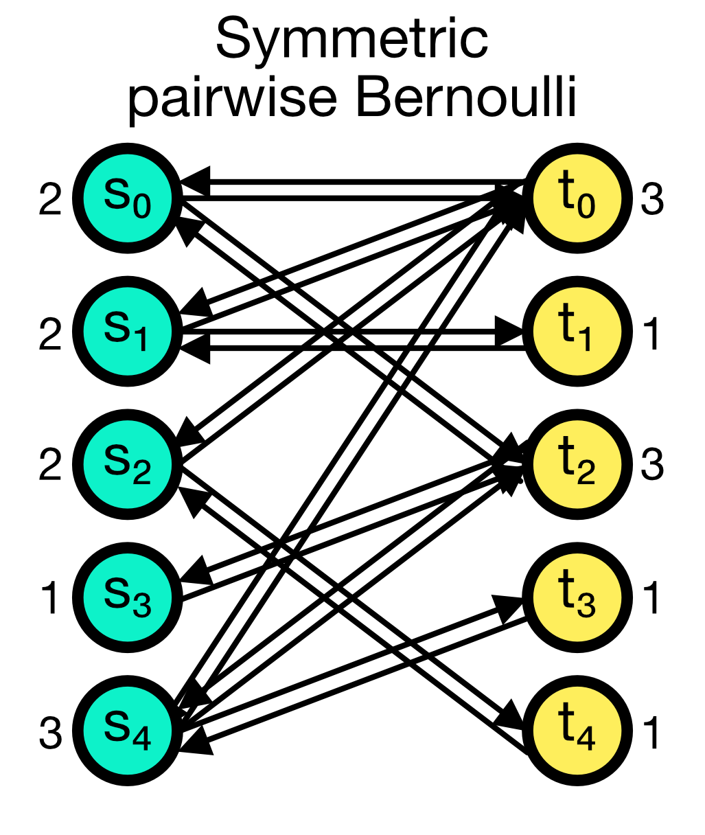
Symmetric pairwise Bernoulli connection scheme in NEST. The connection matrix is symmetric, i.e., if node $i$ is connected to node $j$, then node $j$ is also connected to node $i$ (two connections in total).
Example:
n = 10
m = 12
p = 0.2
S = nest.Create('iaf_psc_alpha', n)
T = nest.Create('iaf_psc_alpha', m)
conn_spec = {'rule': 'symmetric_pairwise_bernoulli', 'p': p,
             'allow_autapses': False, 'make_symmetric': True}
nest.Connect(S, T, conn_spec)
Pairwise Poisson
The pairwise_poisson connection rule establishes connections between the source and target nodes based on a Poisson distribution. The average number of connections pairwise_avg_num_conns is given as an additional parameter. Multiple connections between the same pair of nodes are possible, even for a small average number of connections. Thus, multapses can be established and allow_multapses can not be False.
Example:
n = 10
m = 12
p_avg_num_conns = 0.2 # can be greater than 1
S = nest.Create('iaf_psc_alpha', n)
T = nest.Create('iaf_psc_alpha', m)
conn_spec = {'rule': 'pairwise_poisson',
             'pairwise_avg_num_conns': p_avg_num_conns}
nest.Connect(S, T, conn_spec)
Random, fixed total number
The fixed_total_number connection rule randomly establishes a fixed number of total connections between the source and target nodes. The number of connections N is given as an additional parameter and must be specified. While multapses can be established with this rule, you can also disable them by setting allow_multapses to False.
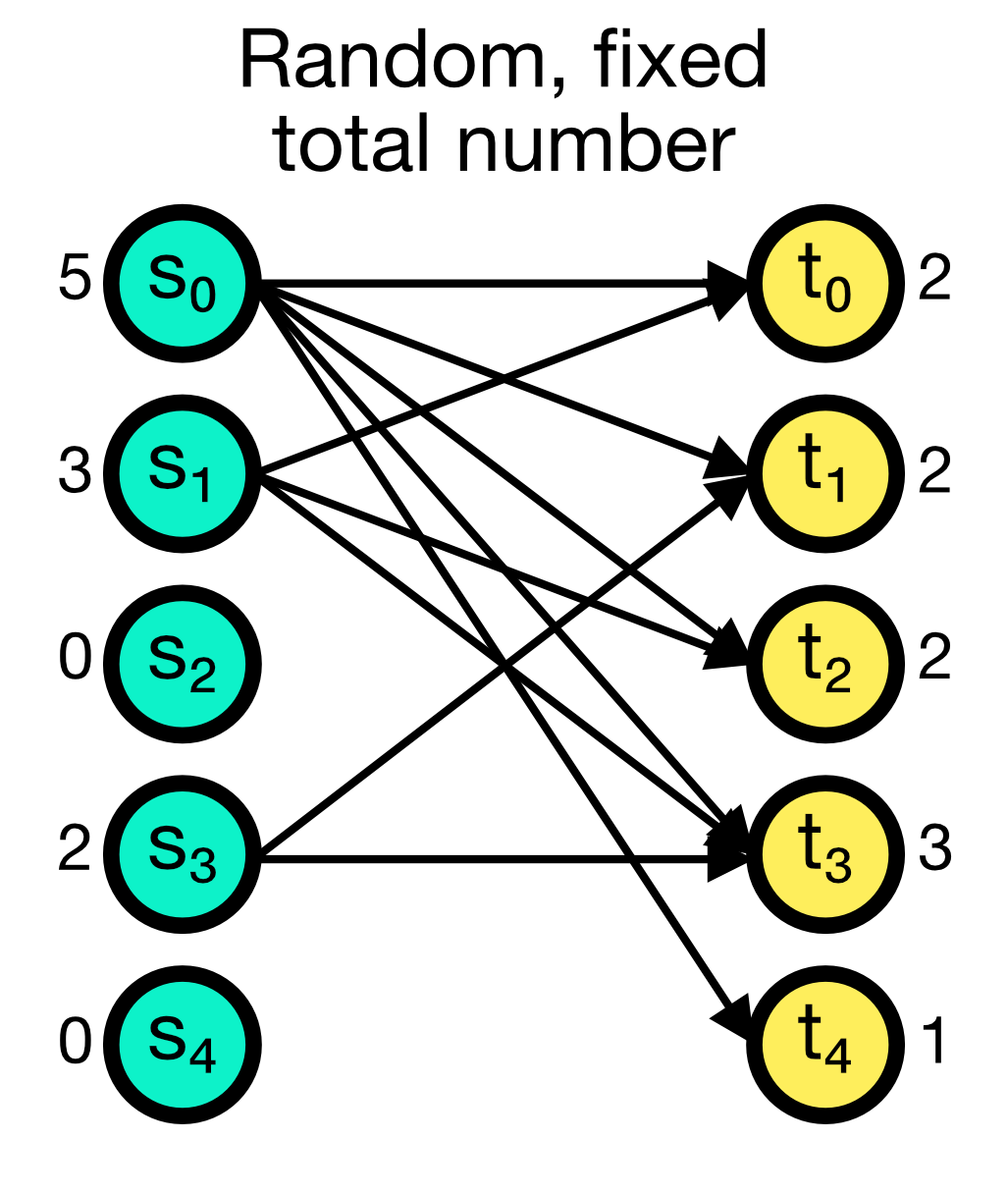
Random, fixed total number connection scheme in NEST. A fixed number of total connections N (here set to 10) is randomly established between the source and target nodes. Multapses can be established with this rule, but you can also disable them.
Example:
n = 5
m = 5
N = 10
S = nest.Create('iaf_psc_alpha', n)
T = nest.Create('iaf_psc_alpha', m)
conn_spec = {'rule': 'fixed_total_number', 'N': N}
nest.Connect(S, T, conn_spec)
Random, fixed in-degree
The fixed_indegree connection rule randomly establishes a fixed number of incoming connections to each target node. The number of incoming connections indegree is given as an additional parameter and must be specified. While multapses can be established with this rule, you can also disable them by setting allow_multapses to False.
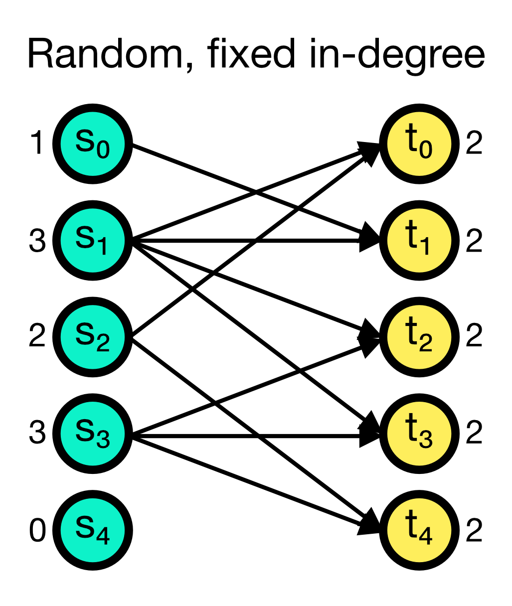
Random, fixed in-degree connection scheme in NEST. A fixed number of incoming connections indegree (here set to 2) is randomly established to each target node. Multapses can be established with this rule, but you can also disable them.
Example:
n = 5
m = 5
N = 2
S = nest.Create('iaf_psc_alpha', n)
T = nest.Create('iaf_psc_alpha', m)
conn_spec = {'rule': 'fixed_indegree', 'indegree': N}
nest.Connect(S, T, conn_spec)
Random, fixed out-degree
The fixed_outdegree connection rule randomly establishes a fixed number of outgoing connections from each source node. The number of outgoing connections outdegree is given as an additional parameter and must be specified. While multapses can be established with this rule, you can also disable them by setting allow_multapses to False.
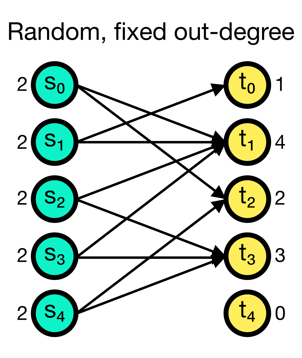
Random, fixed out-degree connection scheme in NEST. A fixed number of outgoing connections outdegree (here set to 2) is randomly established from each source node. Multapses can be established with this rule, but you can also disable them.
Example:
n = 5
m = 5
N = 2
S = nest.Create('iaf_psc_alpha', n)
T = nest.Create('iaf_psc_alpha', m)
conn_spec = {'rule': 'fixed_outdegree', 'indegree': N}
nest.Connect(S, T, conn_spec)
Tripartite Bernoulli with pool
For each possible pair of nodes from a source node collection $S$ and a target node collection $T$, a primary connection is created with probability p_primary. For each primary connection, a third-party connection pair involving a node from a third node collection, e.g., an astrocyte population $A$, is created with the conditional probability p_third_if_primary. This connection pair includes a connection from the $S$ node to the $A$ node, and a connection from the $A$ node to the $T$ node. The $A$ node to connect to is chosen at random from a pool, a subset of the nodes in $A$. By default, this pool is all of $A$.
The pool_type parameter controlls the pool formation and can be random (default) or block. The pool_size parameter must be between 1 and the size of $A$ (default). For random pools, for each node from $T$, pool_size nodes from $A$ are chosen randomly without replacement.
For block pools, two variants exist. Let N_T and N_A be the number of nodes in $T$ and $A$, respectively. If pool_size == 1, the first N_T/N_A nodes in $T$ are assigned the first node in $A$ as their pool, the second N_T/N_A nodes in $T$ the second node in $A$ and so forth. In this case, N_T must be a multiple of N_A. If pool_size > 1, the first pool_size elements of $A$ are the pool for the first node in $T$, the second pool_size elements of $A$ are the pool for the second node in $T$ and so forth. In this case, N_T * pool_size == N_A is required.
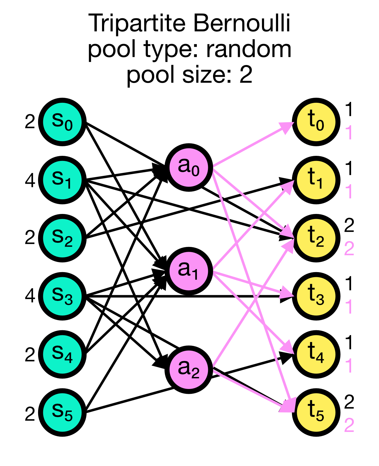
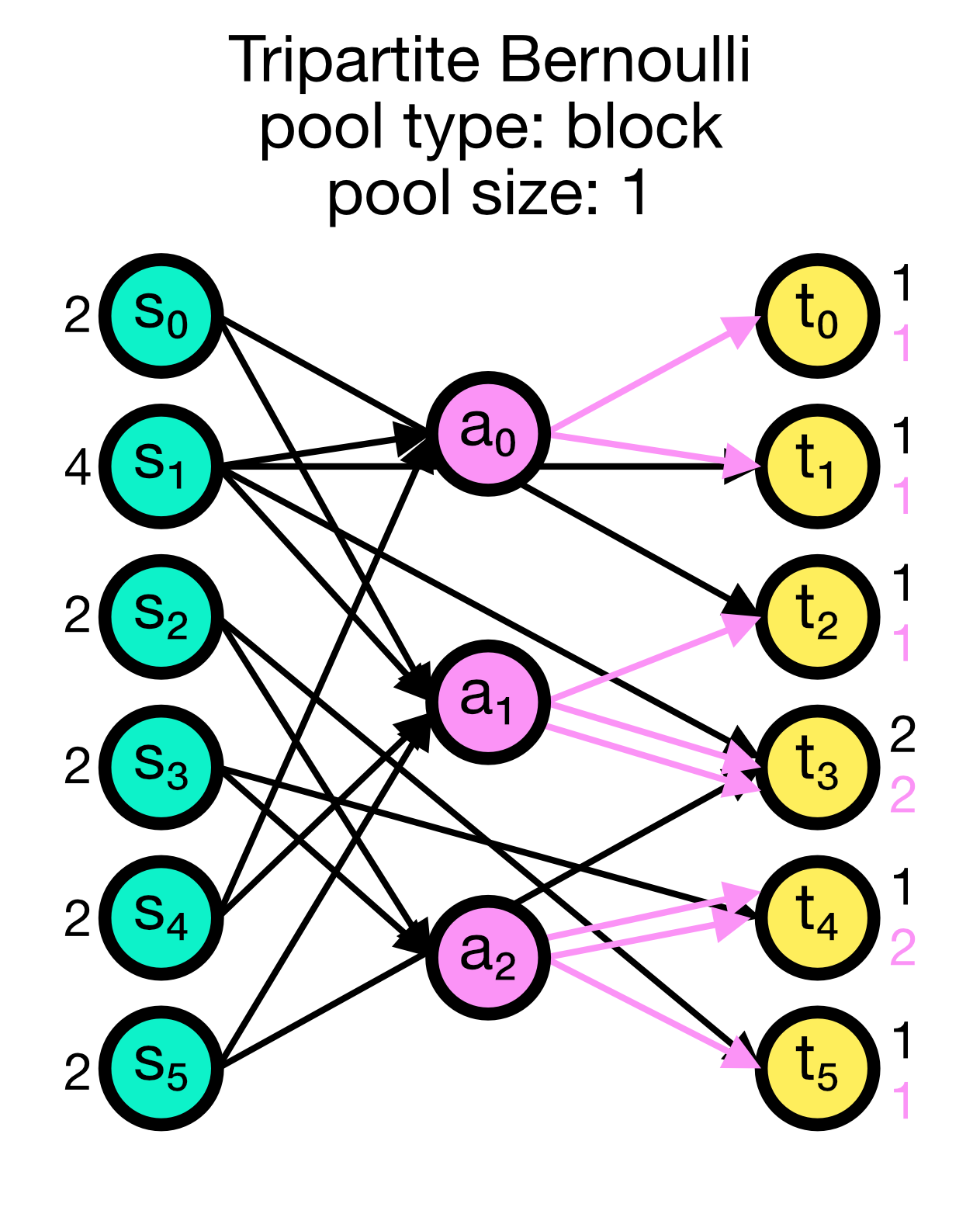
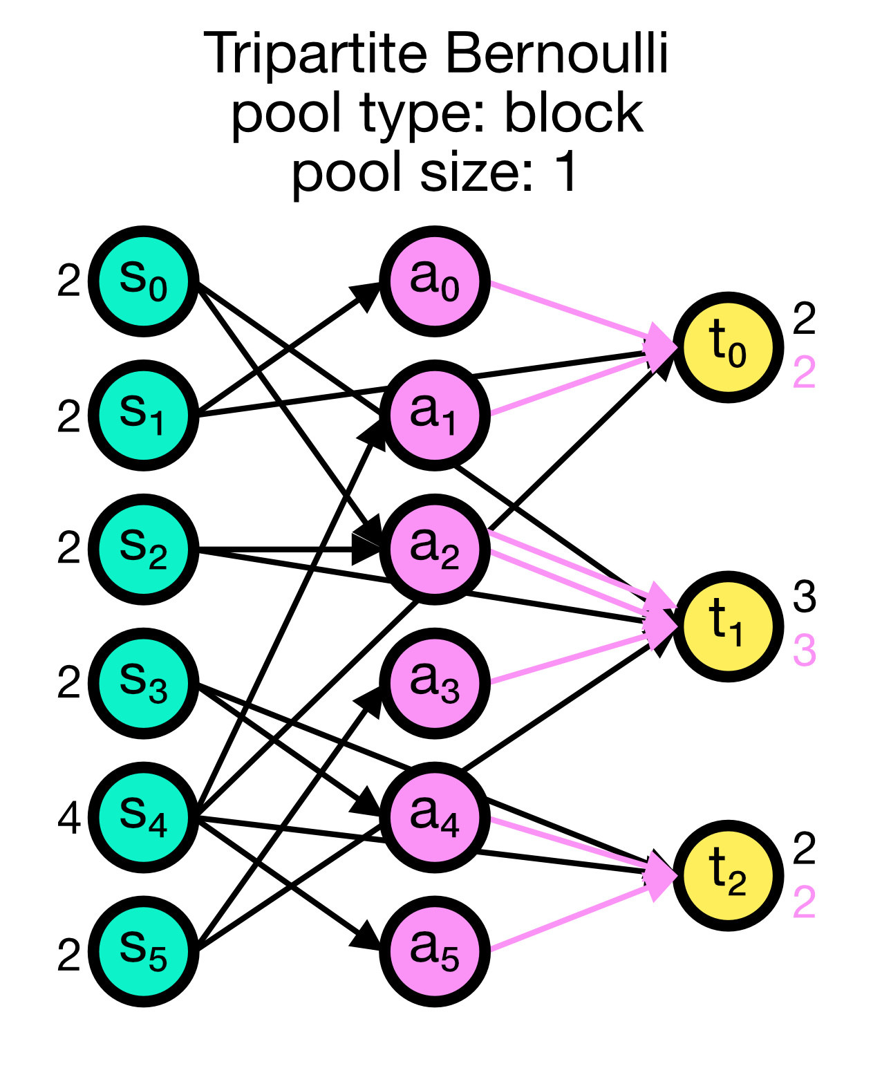
Tripartite Bernoulli connection scheme in NEST. Three different use cases are show with pool_type set to ‘random’ (left) and ‘block’ (middle and right). All cases have a primary connection probability p_primary of 0.2 and a conditional connection probability p_third_if_primary of 1.0. The pool size set to 2 (left and right case) and 1 (middle case), respectively. In the left case, the pool is formed randomly, each node in T can be connected with up to two randomly selected nodes in A. In the middle case, the pool is formed in a block-wise manner, each node in T is connected to one node in A, and each node in A can be connected with up to two nodes in T. In the right case, the pool is also formed in a block-wise manner, but each node in T is now connected to up to two nodes in A, and each node in A can be connected to one nodes in T.
The corresponding code snippet for each of the presented cases above is:
# left plot: random pool
N_S = 6
N_T = 6
N_A = 3
p_primary = 0.2
p_third_if_primary = 1.0
pool_type = 'random'
pool_size = 2
S = nest.Create('aeif_cond_alpha_astro', N_S)
T = nest.Create('aeif_cond_alpha_astro', N_T)
A = nest.Create('astrocyte_lr_1994', N_A)
conn_spec = {'rule': 'tripartite_bernoulli_with_pool',
                  'p_primary': p_primary,
                  'p_third_if_primary': p_third_if_primary,
                  'pool_type': pool_type,
                  'pool_size': pool_size}
syn_specs = {'third_out': 'sic_connection'}
nest.TripartiteConnect(S, T, A, conn_spec, syn_specs)
# middle plot: block pool, pool_size = 1
N_S = 6
N_T = 6
N_A = 3
p_primary = 0.2
p_third_if_primary = 1.0
pool_type = 'block'
pool_size = 1
S = nest.Create('aeif_cond_alpha_astro', N_S)
T = nest.Create('aeif_cond_alpha_astro', N_T)
A = nest.Create('astrocyte_lr_1994', N_A)
conn_spec = {'rule': 'tripartite_bernoulli_with_pool',
             'p_primary': p_primary,
             'p_third_if_primary': p_third_if_primary,
             'pool_type': pool_type,
             'pool_size': pool_size}
syn_specs = {'third_out': 'sic_connection'}
nest.TripartiteConnect(S, T, A, conn_spec, syn_specs)
# right plot: block pool, pool_size > 1
N_S = 6
N_T = 3
N_A = 6
p_primary = 0.2
p_third_if_primary = 1.0
pool_type = 'block'
pool_size = 2
S = nest.Create('aeif_cond_alpha_astro', N_S)
T = nest.Create('aeif_cond_alpha_astro', N_T)
A = nest.Create('astrocyte_lr_1994', N_A)
conn_spec = {'rule': 'tripartite_bernoulli_with_pool',
             'p_primary': p_primary,
             'p_third_if_primary': p_third_if_primary,
             'pool_type': pool_type,
             'pool_size': pool_size}
syn_specs = {'third_out': 'sic_connection'}
nest.TripartiteConnect(S, T, A, conn_spec, syn_specs)
sic_connectionꜛ is a synapse model that is used to connect third-party nodes such as astrocytes to the source and target nodes.
Conclusion
NEST allows for the creation of complex neural networks by providing a variety of connection rules. These rules can be used to establish connections between different types of nodes, such as neurons and astrocytes. The connection rules can be deterministic or probabilistic, and they can be used to create different types of network structures. By using the appropriate connection rules, you can create networks that mimic the connectivity patterns found in the brain and study the dynamics of these networks.
In the next post, we will create a simple neural network using the connection concepts discussed here and explore the dynamics of the network using the NEST simulator.
References and useful links
- Gewaltig, M.-O., & Diesmann, M., NEST (NEural Simulation Tool), 2007 Scholarpedia, 2(4), 1430, doi: 10.4249/scholarpedia.1430ꜛ
- Documentation of the NEST simulatorꜛ
- PyNEST API listingꜛ
- List of all supported neuron and synapse models in NESTꜛ
- Connection concepts in NESTꜛ
- Synapse specification in NESTꜛ
- Senk, Kriener, Djurfeldt, Voges, Jiang, Schüttler, Gramelsberger, Diesmann, Plesser, van Albada, Connectivity concepts in neuronal network modeling, 2022, PLOS Computational Biology, Vol. 18, Issue 9, pages e1010086, doi: 10.1371/journal.pcbi.1010086ꜛ
- Djurfeldt, The Connection-set Algebra—A Novel Formalism for the Representation of Connectivity Structure in Neuronal Network Models, 2012, Neuroinformatics, Vol. 10, Issue 3, pages 287-304, doi: 10.1007/s12021-012-9146-1
- Daniel Hjertholm, Statistical tests for connection algorithms for structured neural networks, 2013, Master’s thesis, Norwegian University of Life Sciences ,Ås, Norway. PDFꜛ




comments