Simulating spiking neural networks with Izhikevich neurons

The Izhikevich neuron model that we have discussed earlier is known for its simplicity and computational efficiency as well as for its biological plausibility. The model is based on two coupled differential equations that describe the membrane potential and the recovery variable of a neuron. The model can reproduce a wide range of spiking behaviors observed in real neurons, such as regular spiking, fast spiking, chattering, and more. In this post, we explore how we can quickly set up a spiking neural network (SNN) simulation using the Izhikevich neuron model in Python.

Spiking neural network (SNN) with Izhikevich neurons, including two different types of neurons (inhibitory and excitatory). The network is simulated using the Izhikevich neuron model in Python as described below.

Spiking Neural Networks (SNNs)

Spiking Neural Networks (SNNs) represent a class of artificial neural networks that closely emulate the neuronal dynamics observed in the biological brain. Unlike traditional artificial neural networks (ANNs) that process information through continuous signals and utilize activation functions like ReLU or sigmoid, SNNs operate on a different principle. Neurons within an SNN communicate via discrete spikes, firing only when their membrane potential exceeds a specific threshold. This spike-based communication is event-driven, mirroring the way biological neurons interact.

This fundamental difference in information processing not only enhances the biological plausibility of SNNs but also contributes to their computational efficiency. In SNNs, the absence of constant signal transmission reduces power consumption, making them particularly suitable for energy-efficient computing in fields like robotics and embedded systems.

Model concept

Let’s recall the basic concept of the Izhikevich neuron model. The model is based on two coupled differential equations that describe the membrane potential $v$ and the recovery variable $u$ of a neuron:

\[\begin{align} \frac{dv}{dt} &= 0.04v^2 + 5v + 140 - u + I \label{eq:model1} \\ \frac{du}{dt} &= a(bv - u) \label{eq:model2} \end{align}\]

with the after-spike reset condition:

\[\begin{align} \text{if } v \geq 30 \text{ mV, then } & \begin{cases} v \leftarrow c \\ u \leftarrow u + d \end{cases} \label{eq:reset} \end{align}\]

The membrane potential $v$ in Eq. ($\ref{eq:model1}$) represents the voltage across the cell membrane, while the recovery variable $u$ in Eq. ($\ref{eq:model2}$) accounts for the activation of the potassium ionic currents. The parameters $a$, $b$, $c$, and $d$ determine the dynamics of the neuron (for a detailed description, please refer to the previous post). The reset condition Eq. ($\ref{eq:reset}$) ensures that the membrane potential is reset to a specific value $c$ after a spike (i.e., after reaching the threshold of 30 mV), and the recovery variable $u$ is increased by a constant $d$. The input current $I$ represents the sum of all incoming synaptic currents and external inputs.

Connectivity matrix

In order to simulate a network of Izhikevich neurons, we need to extend this model to multiple neurons and define the synaptic connections between them. The network structure can be represented by a connectivity matrix $S$, where $S_{ij}$ denotes the synaptic weight from a presynaptic neuron $j$ to a postsynaptic neuron $i$. In this matrix:

• positive values ($S_{ij}>0$) indicate excitatory synaptic connections, meaning that the presynaptic neuron’s firing tends to increase the postsynaptic neuron’s membrane potential, making it more likely to fire.
• negative values ($S_{ij}<0$) indicate inhibitory synaptic connections, where the presynaptic neuron’s firing reduces the postsynaptic neuron’s likelihood of firing by lowering its membrane potential.

This connectivity matrix $S$ not only determines the presence and absence of synaptic connections but also quantifies their strength, profoundly influencing the network dynamics. The overall behavior of the network – such as its ability to exhibit patterns like synchronization, oscillations, or even chaotic activity – depends on the layout and weights of these connections.

In our simulation, we will initialize the synaptic weights randomly, reflecting the diverse connectivity patterns observed in biological neural networks.

Neuron types

In order to make the simulation more realistic, we will also consider two types of neurons in our network: excitatory ($N_e$) and inhibitory neurons ($N_i$). We will implement these neurons types in such a way, that they differ in their intrinsic properties, such as the parameters $a$, $b$, $c$, and $d$ of the Izhikevich model (in our code, we achieve this by adding for each neuron of each type a random value to the respective parameter). By assigning different parameter values to these neuron types, we can capture the diverse spiking behaviors observed in biological neural networks. And of course you can add more neuron types to the network, each with its own set of parameters.

In our simulation code, we will initialize the network with 800 excitatory and 200 inhibitory neurons which reflects the common ratio of excitatory to inhibitory neurons in the mammalian cortex (4:1).

Input current

The time dependent input current $I=I(t)$ in the network is a critical component that drives neuronal activity. It is composed of external inputs and the synaptic currents derived from other neurons within the network. Each neuron’s input current is calculated by summing the products of the synaptic weights $S$ and the membrane potentials $v$ of all presynaptic neurons:

\[\begin{equation} I_i(t) = I_{\text{external}, i}(t) + \sum_{j=1}^{N} S_{ij} \cdot v_j(t) \label{eq:input_current} \end{equation}\]

where:

• $I_i(t)$ is the total input current to neuron $i$ at time $t$,
• $I_{\text{external}, i}(t)$ represents external inputs to neuron $i$, which could include random noise or specific stimuli patterns,
• $S_{ij}$ is the synaptic weight from neuron $j$ to neuron $i$,
• $v_j(t)$ is the membrane potential of the presynaptic neuron $j$,
• $N$ is the total number of neurons in the network.

In our simulation, we enhance the realism by incorporating random noise in the external inputs, reflecting the variability observed in biological neural systems. This approach enables the simulation to exhibit complex network dynamics, such as synchronous firing, oscillations, and potentially chaotic behaviors.

Additionally, in our implementation, $I(t)$ is calculated such that only neurons whose membrane potential $v$ exceeded the threshold in the previous time-step contribute to the input current of other neurons at the current time-step. This event-driven mechanism ensures that the network dynamics are not just reactive to the current state of neuronal activations but are influenced by recent spiking activity, mimicking the temporal dynamics seen in real neural circuits.

Network simulation

The Python code below covers all concepts described above and is based on Izhikevich’s originally published Matlab codeꜛ:

import numpy as np
import matplotlib.pyplot as plt

# for reproducibility:
np.random.seed(0) #100

# simulation time:
T = 1000  # ms

# constants:
Ne = 800  # Number of excitatory neurons
Ni = 200  # Number of inhibitory neurons

# initialize parameters; pre-define parameters for different neuron types:
re = np.random.rand(Ne, 1) # excitatory neurons, "r" stands for random
ri = np.random.rand(Ni, 1) # inhibitory neurons
p_RS  = [0.02, 0.2, -65, 8, "regular spiking (RS)"] # regular spiking settings for excitatory neurons (RS)
p_IB  = [0.02, 0.2, -55, 4, "intrinsically bursting (IB)"] # intrinsically bursting (IB)
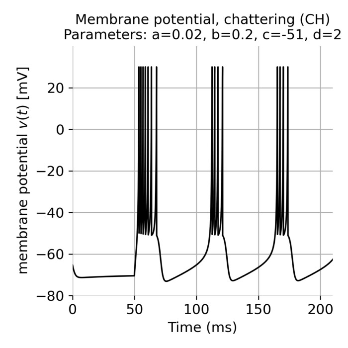
p_CH  = [0.02, 0.2, -51, 2, "chattering (CH)"] # chattering (CH)
p_FS  = [0.1, 0.2, -65, 2, "fast spiking (FS)"] # fast spiking (FS)
p_TC  = [0.02, 0.25, -65, 0.05, "thalamic-cortical (TC)"] # thalamic-cortical (TC) (doesn't work well)
p_LTS = [0.02, 0.25, -65, 2, "low-threshold spiking (LTS)"] # low-threshold spiking (LTS)
p_RZ  = [0.1, 0.26, -65, 2, "resonator (RZ)"] # resonator (RZ)
a_e, b_e, c_e, d_e, name_e = p_RS
a_i, b_i, c_i, d_i, name_i = p_LTS
a = np.vstack((a_e * np.ones((Ne, 1)), a_i + 0.08 * ri))
b = np.vstack((b_e * np.ones((Ne, 1)), b_i - 0.05 * ri))
c = np.vstack((c_e + 15 * re**2,       c_i * np.ones((Ni, 1))))
d = np.vstack((d_e-6 * re**2,          d_i * np.ones((Ni, 1))))
S = np.hstack((0.5 * np.random.rand(Ne+Ni, Ne), -1*np.random.rand(Ne+Ni, Ni)))

# initial values of v and u:
v = -65 * np.ones((Ne+Ni, 1))
u = b * v
firings = np.array([]).reshape(0, 2)  # Spike timings

# initialize variables for recording data:
I_array = np.zeros((Ne+Ni, T))
v_array = np.zeros((Ne+Ni, T))
u_array = np.zeros((Ne+Ni, T))

# simulation of 1000 ms:
for t in range(0, T):
    # step 1: input current calculation:
    # i.e., calculate input current for each neuron with noise contribution (this is our "I_external(t)").
    I = np.vstack((5 * np.random.randn(Ne, 1), 2 * np.random.randn(Ni, 1)))
    # summing synaptic contributions if there are any fired neurons in previous time step:
    if t > 0:  
        I += np.sum(S[:, fired], axis=1).reshape(-1, 1)
        
    # step 2: update the membrane potential and recovery variable (neuron dynamics) with Euler's method:
    v += 0.5 * (0.04 * v**2 + 5 * v + 140 - u + I)
    v += 0.5 * (0.04 * v**2 + 5 * v + 140 - u + I)
    u +=  a * (b * v - u)
    
    # step 3: check for spikes and update the membrane potential and recovery variable:
    fired = np.where(v >= 30)[0] # check if the membrane potential exceeds 30 mV
    if fired.size > 0:
        firings = np.vstack((firings, np.hstack((t * np.ones((fired.size, 1)), fired.reshape(-1, 1)))))
        # equalize all spikes at 30 mV by resetting v first to +30 mV and then to c:
    v[fired] = c[fired] # reset v for fired neurons
    u[fired] = u[fired] + d[fired] # increment u for fired neurons
    
    # step 4: record data:
    I_array[:, t] = I.flatten()
    v_array[:, t] = v.flatten()
    u_array[:, t] = u.flatten()

# plotting the spike timings:
plt.figure(figsize=(7, 7))
plt.scatter(firings[:, 0], firings[:, 1], s=1, c='k')
excitatory = firings[:, 1] < Ne
inhibitory = firings[:, 1] >= Ne
plt.axhline(y=Ne, color='k', linestyle='-', linewidth=1)
plt.text(0.8, 0.76, 'excitatory', color='k', fontsize=12, ha='left', va='center', transform=plt.gca().transAxes, bbox=dict(facecolor='white', alpha=1)) 
plt.text(0.8, 0.84, 'inhibitory', color='k', fontsize=12, ha='left', va='center', transform=plt.gca().transAxes, bbox=dict(facecolor='white', alpha=1))

plt.xlabel('Time (ms)')
plt.ylabel('Neuron index')
plt.xlim([0, T])
plt.ylim([0, Ne+Ni])
plt.yticks(np.arange(0, Ne+Ni+1, 200))
plt.tight_layout()
plt.show()

The code above shows the core concept of the network model simulation. The entire code can be found in this Github repositoryꜛ.

Simulation results

As a first simulation run, we replicate Izikevich’s original example and consider a network with 800 excitatory neurons simulated as regular spiking neurons (RS) and 200 inhibitory neurons simulated as low-threshold spiking neurons (LTS). The simulation is run for 1000 ms. The following plot shows the spike events of each neuron in the network as a function of time:

Spike events of each neuron in the network as a function of time. The network consists of 800 excitatory neurons (regular spiking, RS) and 200 inhibitory neurons (low-threshold spiking, LTS), separated by the horizontal line.

What we can observe in this simulation is that, for occasionally episodes, a synchronous firing pattern emerges in the network, where groups of neurons fire together in a coordinated manner. These episodes repeat with a frequency of about 10 Hz (first three peaks in the plot) and about 40 Hz (remaining peaks). This behavior is the exact replication of what Izhikevich simulated in his original work, which associates these firing patterns with the brain’s alpha and gamma oscillations, respectively. Between these episodes, the network exhibits a more irregular, Poisson-like firing pattern. The observed firing patterns demonstrate the network’s ability to exhibit complex spiking dynamics, even though the neurons in the network are connected randomly and no synaptic plasticity rules are implemented. The neurons organize themselves into synchronous firing patterns or assemblies, exhibiting a collective rhythmic behavior. And according to Izhikevich, this rhythmic behavior corresponds to that of the mammalian cortex in awake states.

Let’s also take a look at the corresponding input currents of each neuron in the network:

Corresponding input currents of each neuron in the network as a function of time.

We can see, how the inputs currents of the neuron peak synchronously with the observed clusters of spiking events. This synchronous behavior is a result of the network’s connectivity and the synaptic weights between the neurons. In our model, the input current $I$ for each neuron includes contributions from the spikes of other neurons, as defined by the connectivity matrix $S$ (compare Eq. ($\ref{eq:input_current}$)). This means that when a neuron fires (its membrane potential $v$ surpasses the threshold), it influences the input currents of other neurons according to the synaptic weights specified in $S$. If $S_{ij}$ is positive (excitatory connection), it will increase the input current $I_{i}$ of neuron $i$ when neuron $j$ spikes. If $S_{ij}$ is negative (inhibitory connection), it will decrease $I_{i}$. If there are episodes of synchronous firing, where many neurons fire (nearly) simultaneously, these spiking events contribute collectively to significant peaks in the input currents of neurons connected to them. And this exactly what we observe in the plot above.

This synchronous behavior between spikes and input currents is an important aspect of how neural networks function, both in biological and artificial contexts. It underscores the interconnected nature of neurons, where the action of one neuron can influence many others, leading to complex behaviors such as oscillations, waves of activity, and even synchronized firing patterns seen in various neural processes and disorders.

Finally, let’s take a brief look at the membrane potential and recovery variable traces of one exemplary excitatory neuron (blue) and an inhibitory neuron (orange) in the network:

Voltage (two upper panels) and recovery variable traces (two lower panels) of an exemplary excitatory neuron (blue) and an inhibitory neuron (orange) in the network.

The plots show Poisson-like spiking patterns of both neuron types along with distinct spiking events that correlate with the spiking clusters within the network. The recovery variable $u$ of the inhibitory neuron (orange) exhibits a different behavior with lower amplitudes compared to the excitatory neuron (blue). This difference in the recovery variable dynamics is a result of the different parameter values assigned to the two neuron types, reflecting the ability to assign diverse spiking behaviors to different neuron populations in the network.

Altering the connectivity within the network

By altering the synaptic weights in the connectivity matrix $S$, we can observe how the network dynamics change and generates different spiking patterns. For instance, we run the simulation for four different scenarios with varying excitatory and inhibitory synaptic weights defined as follows, while keeping the other parameters constant:

# define various synaptic weights for different scenarios (uncomment one of the following):
S = np.hstack((0.60 * np.random.rand(Ne+Ni, Ne), -1.6*np.random.rand(Ne+Ni, Ni))) # S1
#S = np.hstack((0.60 * np.random.rand(Ne+Ni, Ne), -0.6*np.random.rand(Ne+Ni, Ni))) # S2
#S = np.hstack((0.30 * np.random.rand(Ne+Ni, Ne), -0.1*np.random.rand(Ne+Ni, Ni))) # S3
#S = np.hstack((0.10 * np.random.rand(Ne+Ni, Ne), -0.1*np.random.rand(Ne+Ni, Ni))) # S4

• Scenario 1 (S1): Strong excitatory and strong inhibitory synaptic weights
• Scenario 2 (S2): Strong excitatory and weak inhibitory synaptic weights
• Scenario 3 (S3): Weak excitatory and very weak inhibitory synaptic weights
• Scenario 4 (S4): Very weak excitatory and very weak inhibitory synaptic weights

Spike events of each neuron in the network as a function of time in response to different synaptic weights scenarios S1 (top left), S2 (top right), S3 (bottom left), and S4 (bottom right). Note that the terms “inhibitory” and “excitatory” are no longer appropriate for the given scenarios, but I kept them to distinguish the two different types of neurons in the simulations.

By increasing both the excitatory and inhibitory synaptic weights (S1) (compared to Izhikevich’s original set-up), we observe a more synchronized firing pattern in the network. This synchronous behavior is due to the stronger synaptic connections, which lead to more pronounced interactions between neurons. However, the frequency of the synchronous firing episodes has now changed. By decreasing the inhibitory synaptic weights (S2), the firing patterns change even more dramatically, with less frequent and longer-lasting synchronous firing episodes of heavily synchronized neurons. If we additionally decrease the excitatory synaptic weights (S3), the frequency of synchronous firing episodes becomes higher and, as expected, the synchronicity between neurons decreases. Finally, by setting both excitatory and inhibitory synaptic weights to very low values (S4), the network exhibits a more irregular firing pattern with almost no recognizable synchronicity between neurons.

These results demonstrate how the network dynamics are shaped by the synaptic weights and how different connectivity patterns can lead to distinct spiking behaviors. By adjusting the synaptic weights, we can observe a wide range of network behaviors, from synchronous firing to irregular spiking patterns, reflecting the diverse dynamics observed in biological neural networks.

Changing the neuron types

In addition to altering the synaptic weights, we can also change the neuron types in the network to observe how different spiking behaviors emerge. As an example, we simulate a network with

• regular spiking (RS) and chattering (CH) neurons (combination 1),
• regular spiking (RS) and thalamic-cortical (TC) neurons (combination 2),
• resonator (RZ) and regular spiking (RS) neurons (combination 3), and
• intrinsically bursting (IB) and intrinsically bursting (IB) neurons (combination 4).

We assign different connectivity matrices $S$ to these simulations in order to enhance emerging spiking patterns. We use the connectivity scenarios defined in the previous section and define the following additional scenario S5:

S = np.hstack((0.30 * np.random.rand(Ne+Ni, Ne), -0.2*np.random.rand(Ne+Ni, Ni))) # S5

Spike events of each neuron in the network as a function of time in response to different neuron types combinations: RS and CH with synaptic connectivity scenario S5 (top left), RS and TC with synaptic connectivity scenario S5 (top right), RZ and RS with synaptic connectivity scenario S3 (bottom left), and IB and IB with synaptic connectivity scenario S4 (bottom right). Again, the terms “inhibitory” and “excitatory” are no longer appropriate for the given scenarios, but I kept them to distinguish the two different types of neurons in the simulations.

By simulating various neuron type combinations, we can observe a wide range of spiking behaviors in the network, each exposing distinct firing patterns. It demonstrates how the intrinsic properties of neurons, such as their parameter values in the Izhikevich model, can shape the network dynamics and lead to diverse spiking behaviors. By combining different neuron types and synaptic weights, we can explore the rich repertoire of spiking patterns that can emerge in neural networks, reflecting the complexity and adaptability of biological neural systems.

Conclusion

In this exploration of the Izhikevich neuron model applied to spiking neural networks (SNNs), we’ve showcased its capability to simulate complex neural dynamics that mirror biological processes. Renowned for its simplicity, computational efficiency, and biological plausibility, the Izhikevich model is an exceptional tool for understanding how neuronal interactions within neural networks lead to phenomena like synchronous firing and oscillatory behaviors. Furthermore, due to its computational efficiency, the Izhikevich SNN enables real-time processing, making it suitable for applications in computational neuroscience without compromising biological realism.

By adjusting network parameters and connectivity, we’ve demonstrated how different neuronal behaviors can be elicited, which enhances our understanding of neural circuit functionality and adaptability. Moving forward, integrating mechanisms like synaptic plasticity could open new pathways for simulating learning and memory, further bridging the gap between artificial and biological neural systems. The insights gained from these models are invaluable for advancing artificial intelligence and developing new treatments for neurological disorders.

The complete code used in this blog post is available in this Github repositoryꜛ. Feel free to experiment with it, modify the parameters, and explore the dynamics of the Izhikevich SNN model further.

References and further reading

• Izhikevich, Simple model of spiking neurons, 2003, IEEE Transactions on Neural Networks, Vol. 14, Issue 6, pages 1569-1572, doi: 10.1109/TNN.2003.820440ꜛ, PDFꜛ
• Izhikevich, Eugene M., (2010), Dynamical systems in neuroscience: The geometry of excitability and bursting (First MIT Press paperback edition), The MIT Press, ISBN: 978-0-262-51420-0, PDFꜛ