Building a neural network from scratch using NumPy

Ever thought about building you own neural network from scratch by simply using NumPy? In this post, we will do exactly that. We will build a simple feedforward neural network and train it on the MNIST dataset. The MNIST datasetꜛ is a collection of 28x28 pixel grayscale images of handwritten digits (0-9). It is a popular dataset for getting started with machine learning and computer vision. The dataset contains 60,000 training images and 10,000 test images. The goal is to train a model that can correctly classify the images into their respective digit classes.

Building a neural network from scratch using NumPy, applied to the MNIST dataset.

The motivation for this venture was the blog “Simple Neural Network on MNIST Handwritten Digit Datasetꜛ” post by Muhammad Ardi. In his post, Muhammad provides a simple implementation of a neural network using keras. I thought it would be interesting to see how we can achieve the same results by using only NumPy. Let’s see how we can do that.

Preparing the conda environment

Before we start, we need to make sure that we have the necessary packages installed. We will just use NumPy, Matplotlib, and keras for loading the MNIST dataset. Let’s create a new conda environment and install the required packages.

conda create -n numpy_ann python=3.11
conda activate numpy_ann
conda install -y mamba
mamba install -y numpy matplotlib keras ipykernel

If you are using an Apple Silicon chip, follow these instructions to install TensorFlow (TensorFlow is required by keras).

Initializing the neural network

First, we need to initialize the parameters of the neural network. We will use a simple feedforward neural network with one hidden layer. The input layer will have 784 neurons (28x28 pixels), the hidden layer will have 5 neurons, and the output layer will have 10 neurons (one for each digit class):

def initialize_network(input_size, hidden_size, output_size):
    """
    This function initializes the parameters of the neural network.
    W1 and W2 are weight matrices for the input layer and the hidden layer, respectively.
    b1 and b2 are bias vectors for the hidden layer and the output layer, respectively.
    """
    np.random.seed(42)  # for reproducibility
    network = {
        'W1': np.random.randn(input_size, hidden_size) * 0.01,
        'b1': np.zeros((1, hidden_size)),
        'W2': np.random.randn(hidden_size, output_size) * 0.01,
        'b2': np.zeros((1, output_size))
    }
    return network

input_size = 28*28  # MNIST images have 28x28 pixels 
hidden_size = 5  # number of neurons in the hidden layer
output_size = 10  # Number of classes (the digits 0-9)
network = initialize_network(input_size, hidden_size, output_size)

In the defined function above, W1 and W2 are weight matrices for the input layer and the hidden layer, respectively. b1 and b2 are bias vectors for the hidden layer and the output layer, respectively.

Initializing the network parameters is a crucial step. We want to initialize the weights and biases such that the network can learn effectively. We will use small random values for the weights and zeros for the biases. This is a common practice in neural network initialization. The small random values help to break the symmetry of the weights and prevent the network from getting stuck during training.

Forward propagation

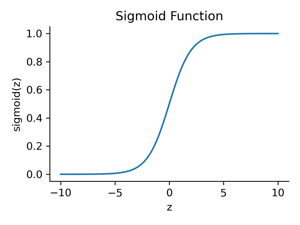
The next step is to implement the forward propagation algorithm. This is the process of computing the output of the network given an input. We will use the sigmoid function,

\[\sigma(z) = \frac{1}{1 + e^{-z}},\]

as the activation function for the hidden layer and the softmax function,

\[\text{softmax}(z) = \frac{e^{z}}{\sum_{i=1}^{n} e^{z_i}},\]

for the output layer:

def sigmoid(z):
    return 1 / (1 + np.exp(-z))

def softmax(z):
    exp_scores = np.exp(z)
    return exp_scores / np.sum(exp_scores, axis=1, keepdims=True)

The sigmoid function.

The feedforward algorithm is implemented as follows:

def feedforward(network, X):
    z1 = X.dot(network['W1']) + network['b1']
    a1 = sigmoid(z1)
    z2 = a1.dot(network['W2']) + network['b2']
    a2 = softmax(z2)
    activations = {
        'a1': a1,
        'a2': a2
    }
    return activations

The feedforward function takes the input X and propagates it through the network to compute the output. It returns the activations of the hidden layer (a1) and the output layer (a2).

Loss function

After defining the forward propagation algorithm, we need to define the loss function. The loss function measures how well the network is performing. We will use the cross-entropy loss function,

Let $a^{[2]}$ be the output of the neural network and $Y$ the actual labels of the dataset, where $m$ is the number of training examples. The cost function $J$ can be formulated as follows:

\[J(a^{[2]}, Y) = -\frac{1}{m} \sum_{i=1}^{m} \left[ Y^{(i)} \log(a^{[2](i)}) + (1 - Y^{(i)}) \log(1 - a^{[2](i)}) \right]\]

with

• $a^{[2](i)}$ the prediction of the network for the $i$th training example.
• $Y^{(i)}$ the actual label of the $i$th training example.
• $\log$ the natural logarithm.
• $\sum_{i=1}^{m}$ the summation running over all $m$ training examples.

The cross-entropy loss which is commonly used for classification problems. It measures the “distance” between the predicted probabilities $a^{[2]}$ and the actual labels $Y$, with the aim of minimizing this distance:

def compute_cost(a2, Y):
    m = Y.shape[0]  # number of examples
    log_probs = np.multiply(np.log(a2), Y) + np.multiply((1 - Y), np.log(1 - a2))
    cost = -np.sum(log_probs) / m
    return cost

The compute_cost function takes the output of the network (a2) and the true labels (Y) and computes the cross-entropy loss.

Backpropagation

Next, we need to implement the backpropagation algorithm. This is the process of computing the gradients of the loss function with respect to the network parameters. These gradients are used to update the parameters during training. Let’s denote again:

• $a^{[1]}$ as the activations from the hidden layer.
• $a^{[2]}$ as the activations (output predictions) from the output layer.
• $Y$ as the actual labels.
• $m$ as the number of examples.
• $W^{[1]}$ and $b^{[1]}$ as the weights and biases for the connections to the hidden layer.
• $W^{[2]}$ and $b^{[2]}$ as the weights and biases for the connections to the output layer.

The backpropagation process calculates the gradient of the cost function with respect to each parameter in the network. The steps are as follows:

1. Calculate the error in the output layer ($dz^{[2]}$):

\[dz^{[2]} = a^{[2]} - Y\]

2. Calculate the gradients for the output layer (Layer 2) weights ($dW^{[2]}$) and biases ($db^{[2]}$):

\[dW^{[2]} = \frac{1}{m} a^{[1]T} dz^{[2]}\] \[db^{[2]} = \frac{1}{m} \sum dz^{[2]}\]

3. Calculate the error in the hidden layer ($dz^{[1]}$):

\[dz^{[1]} = dz^{[2]} W^{[2]T} * a^{[1]} * (1 - a^{[1]})\]

* denotes element-wise multiplication. Here, the operation $a^{[1]} * (1 - a^{[1]})$ applies the derivative of the sigmoid function (since sigmoid was used as the activation function in the hidden layer), which is necessary for the chain rule in backpropagation.

4. Calculate the gradients for the hidden layer (Layer 1) weights ($dW^{[1]}$) and biases ($db^{[1]}$):

\[dW^{[1]} = \frac{1}{m} X^T dz^{[1]}\] \[db^{[1]} = \frac{1}{m} \sum dz^{[1]}\]

The gradients ($dW^{[1]}$, $db^{[1]}$, $dW^{[2]}$, $db^{[2]}$) are then used to update the network’s parameters, aiming to minimize the cost function through gradient descent.

This algorithm can be implemented in Python as follows:

def backpropagate(network, activations, X, Y):
    m = X.shape[0]
    
    # output from the feedforward:
    a1, a2 = activations['a1'], activations['a2']
    
    # error during output:
    dz2 = a2 - Y
    dW2 = (1 / m) * np.dot(a1.T, dz2)
    db2 = (1 / m) * np.sum(dz2, axis=0, keepdims=True)
    
    # error in the hidden layer:
    dz1 = np.dot(dz2, network['W2'].T) * a1 * (1 - a1)
    dW1 = (1 / m) * np.dot(X.T, dz1)
    db1 = (1 / m) * np.sum(dz1, axis=0, keepdims=True)
    
    # gradients:
    gradients = {
        'dW1': dW1,
        'db1': db1,
        'dW2': dW2,
        'db2': db2
    }
    
    return gradients

The backpropagate function takes the input X, the true labels Y, and the activations from the feedforward step. As described above, it computes the gradients of the loss with respect to the parameters of the network and returns the gradients.

Define the main training loop

The last step is to define the main training loop. This loop iterates over the training data and updates the parameters of the network using the gradients computed by the backpropagation algorithm:

def update_parameters(network, gradients, learning_rate):
    network['W1'] -= learning_rate * gradients['dW1']
    network['b1'] -= learning_rate * gradients['db1']
    network['W2'] -= learning_rate * gradients['dW2']
    network['b2'] -= learning_rate * gradients['db2']
    
def train_network(network, X_train, Y_train, X_val, Y_val, num_iterations=1000, learning_rate=0.1):
    train_costs = []
    val_costs = []
    for i in range(num_iterations):
        # training:
        train_activations = feedforward(network, X_train)
        train_cost = compute_cost(train_activations['a2'], Y_train)
        train_costs.append(train_cost)
        gradients = backpropagate(network, train_activations, X_train, Y_train)
        update_parameters(network, gradients, learning_rate)
        
        # validation:
        val_activations = feedforward(network, X_val)
        val_cost = compute_cost(val_activations['a2'], Y_val)
        val_costs.append(val_cost)

        if i % 100 == 0:
            print(f"Costs after iteration {i}: Training {train_cost}, Validation {val_cost}")
    return train_costs, val_costs

The train_network function takes the network parameters, the training data, the validation data, and the hyperparameters of the training process. It iterates over the training data, computes the loss, and updates the parameters of the network using the gradients. It also computes the loss on the validation data and stores the training and validation costs for later analysis.

We can also define a function to make predictions using the trained network. This will help us later to further evaluate the performance of the network on the test data:

def predict(network, X):
    activations = feedforward(network, X)
    predictions = np.argmax(activations['a2'], axis=1)
    return predictions

Loading and pre-processing the MNIST dataset

Now that we have defined the neural network and the training process, we can load the MNIST dataset and train the network. We will use the keras library to load the dataset (the only time we use keras in this example):

(X_train, y_train), (X_test, y_test) = mnist.load_data()

Here some images along with their true labels:

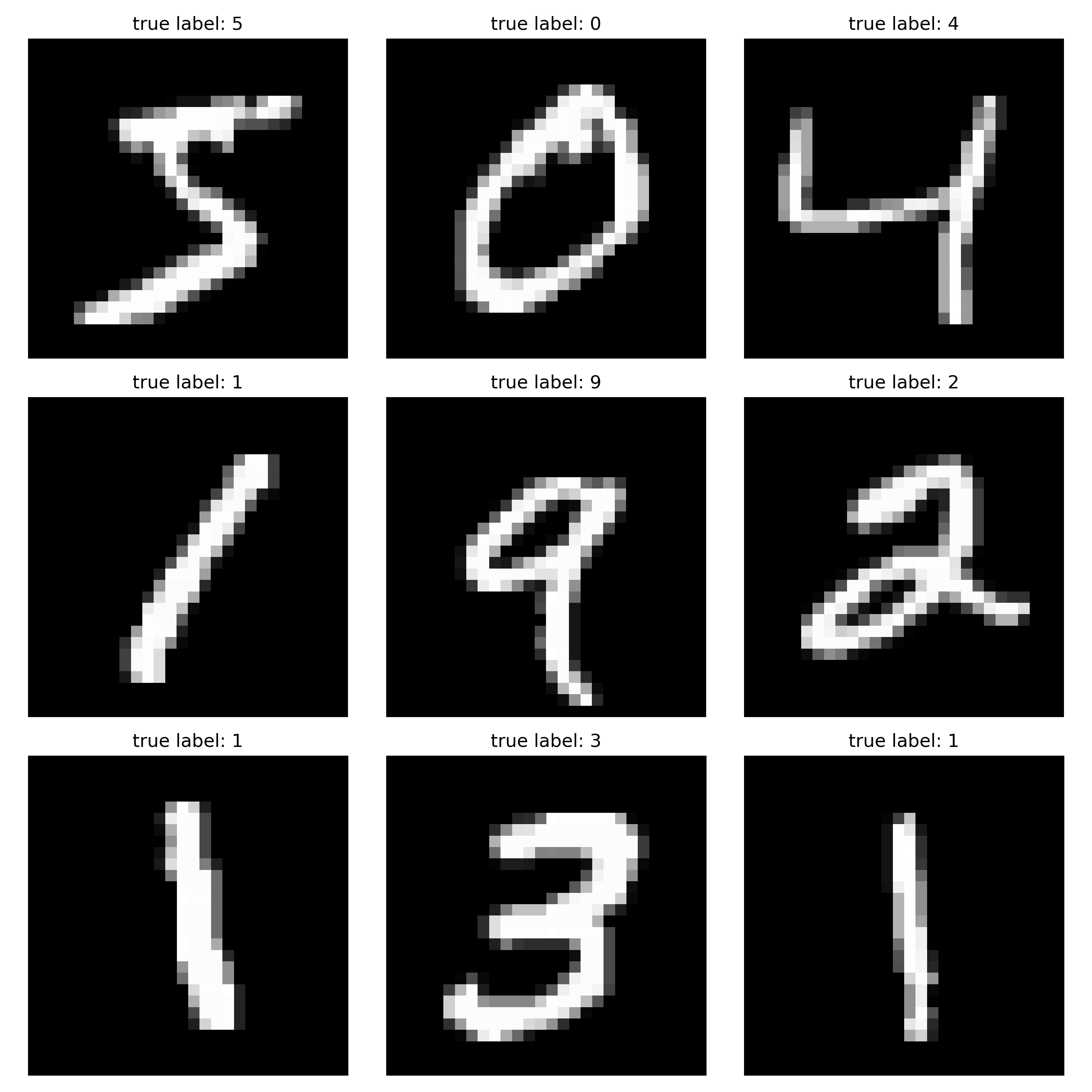Some images from the MNIST dataset along with their true labels.

We need to flatten the input data and normalize it, as the network expects the input to be a vector of pixel values ranging between 0 and 1:

X_train_flat = X_train.reshape(X_train.shape[0], -1) / 255.
X_test_flat  = X_test.reshape(X_test.shape[0], -1) / 255.

We also need to convert the labels to “one-hot” format, as the output layer of the network requires a binary vector for each label. The “one-hot” conversion converts, e.g., the label 3 to [0, 0, 0, 1, 0, 0, 0, 0, 0, 0]:

def convert_to_one_hot(Y, C):
    Y = np.eye(C)[Y.reshape(-1)]
    return Y

num_classes = 10  # number of classes (digits 0-9) in the MNIST dataset
y_train_one_hot = convert_to_one_hot(y_train, num_classes)
y_test_one_hot  = convert_to_one_hot(y_test, num_classes)

Training and validating the network

Now we can train the network using the training data. As hpyerparameters, we will use 1000 iterations and a learning rate of 0.5. You can experiment with different hyperparameters to see how they affect the performance of the network:

# set the hyperparameters:
epochs = 1000 # here, epochs equals the number of iterations since we use the entire dataset for each iteration (no mini-batch)
learning_rate = 0.5

# train the network:
train_costs, val_costs = train_network(network, X_train_flat, 
                                       y_train_one_hot, X_test_flat, y_test_one_hot, 
                                       num_iterations=epochs, learning_rate=learning_rate)

Training the network will take some time, depending on the number of iterations, the learning rate, and the machine you are using. Running the training loop will give you an output similar to the following:

Costs after iteration 0: Training 3.250864945250842, Validation 3.250411860389282
Costs after iteration 100: Training 2.7007775438283583, Validation 2.6767576337216497
Costs after iteration 200: Training 1.8507350583935092, Validation 1.8343369824764788
Costs after iteration 300: Training 1.487676493296171, Validation 1.472138991701572
Costs after iteration 400: Training 1.2611294493021457, Validation 1.2442551904888854
Costs after iteration 500: Training 1.1039540285064955, Validation 1.0883506980077577
Costs after iteration 600: Training 1.0002200773938172, Validation 0.98698917788099
Costs after iteration 700: Training 0.9303917677855934, Validation 0.9192967613186466
Costs after iteration 800: Training 0.8812264423101561, Validation 0.8718480425948801
Costs after iteration 900: Training 0.8447855877156378, Validation 0.8368302438646806

After training, you can plot the training and validation costs to see how the network’s performance changes over time:

fig = plt.figure(figsize=(6, 4))
plt.plot(train_costs, label='Training Loss')
plt.plot(val_costs, label='Validation Loss')
plt.xlabel('iteration')
plt.ylabel('loss')
plt.title('Training and validation loss curves')
plt.gca().spines['top'].set_visible(False)
plt.gca().spines['right'].set_visible(False)
plt.legend()
plt.tight_layout()
plt.show()

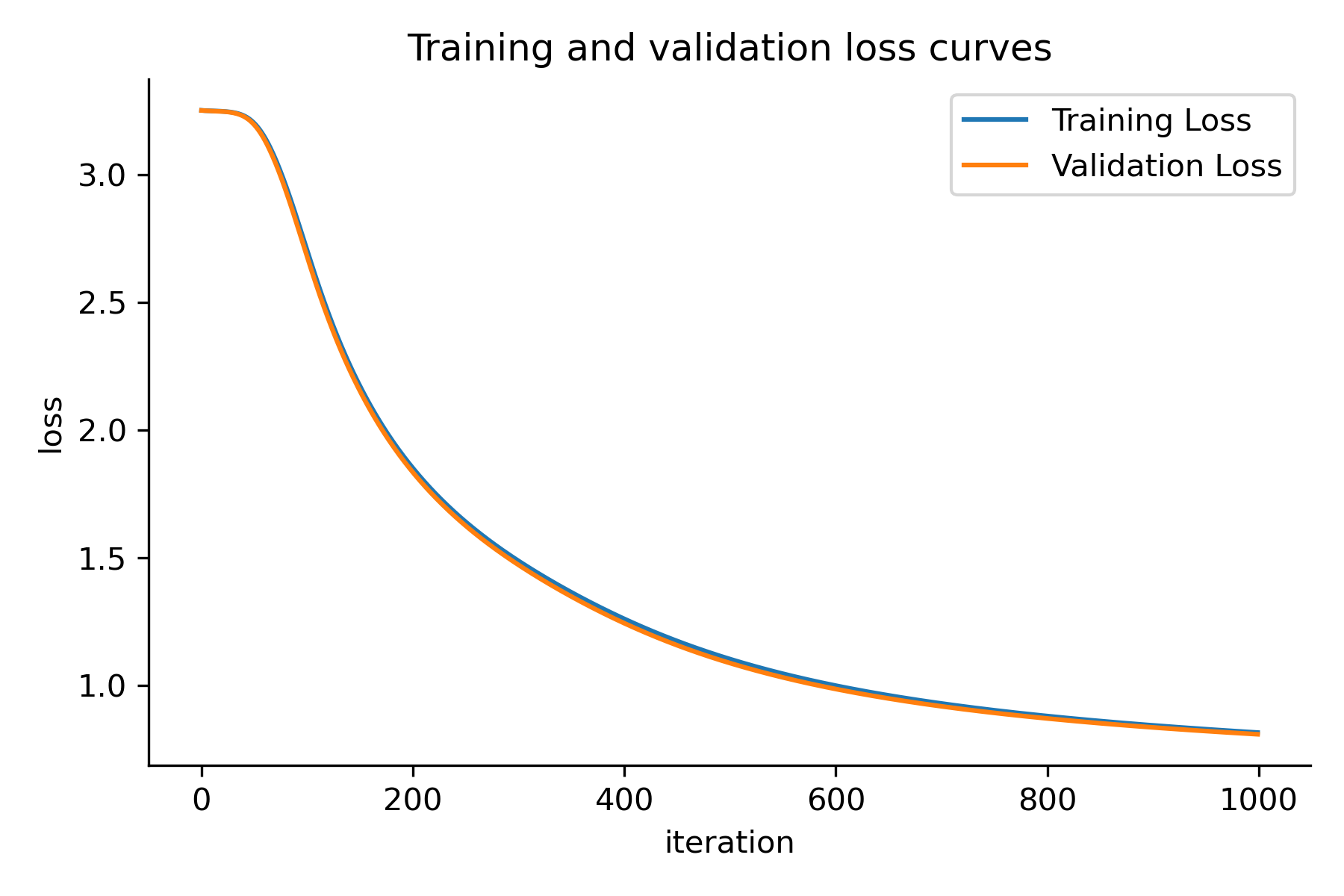The training and validation loss curves.

The plot shows you how the training and validation costs change over the course of the training process. You can use this information to tune the hyperparameters of the network and improve its performance. Since the loss curves are decreasing and the validation loss is close to the training loss, we can assume that the network is learning effectively for the chosen hyperparameters.

In order to further validate the performance of the network, we can make predictions on the test data and compute the accuracy of the network:

# predict the test data:
predictions = predict(network, X_test_flat)

# calculate the accuracy:
actual_labels = y_test
accuracy = np.mean(predictions == actual_labels)
print(f'Accuracy of the network on the test data: {accuracy * 100:.2f}%')

Accuracy of the network on the test data: 86.69%

The accuracy of 86.69% is a good result for our simple feedforward neural network. Feel free to play around with different hyperparameters to see if you can improve the performance further.

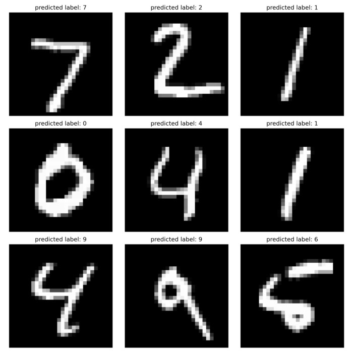
To see, how our model predicts the test data, we can plot some of the test images along with their predicted labels:

fig, axes = plt.subplots(nrows=3, ncols=3, figsize=(10, 10))
for i, ax in enumerate(axes.flat):
	ax.imshow(X_test[i], cmap='gray')
	ax.set_title(f'predicted label: {predictions[i]}')
	ax.axis('off')
plt.show()

Predicted labels for some images from the MNIST dataset.

As we can see, the network is able to correctly classify most of the test images. Some digits are more difficult to classify than others, but overall the network is doing a good job.

Conclusion

I was actually surprised how easy it is to build a simple feedforward neural network from scratch just using NumPy. It also ran quite fast on my machine. The network was able to achieve a good accuracy on the MNIST dataset, which is a good starting point for further experimentation. You can experiment with different network architectures, hyperparameters, and training strategies to improve the performance of the network. You can also try training the network on other datasets to see how it performs on different types of data. Introducing mini-batch training, regularization, and other techniques to improve the performance of the network would also be a good next step.

I hope this post has given a good starting point for a better intuition about how neural networks work and what is happening under the hood when using libraries like keras or TensorFlow. If you have any comments or ideas for other experiments, feel free to share them in the comments below. I would be happy to hear from you.

The complete code used in this post can be found in this GitHub repositoryꜛ.