Mutual information and its relationship to information entropy

Mutual information is an essential measure in information theory that quantifies the statistical dependence between two random variables. Given its broad applicability, it has become an invaluable tool in diverse fields like machine learning, neuroscience, signal processing, and more. This post explores the mathematical foundations of mutual information and its relationship to information entropy. We will also demonstrate its implementation in some Python examples.

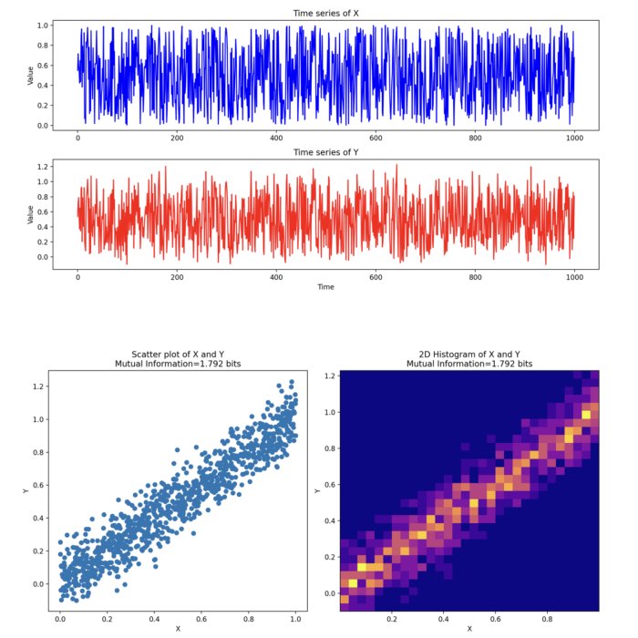
The concept of mutual information and its relation to information entropy

Mutual information (MI) between two random variables is a measure that quantifies the mutual dependence between the two variables. More specifically, it quantifies the expected value of the pointwise mutual information (PMI).

Let $X$ and $Y$ be two discrete random variables. The mutual information $I(X;Y)$ between $X$ and $Y$ can be calculated as:

\[I(X; Y) = \sum_{x} \sum_{y} p(x, y) \log \left( \frac{p(x, y)}{p(x) p(y)} \right)\]

Here, $p(x, y)$ is the joint probability mass function of $X$ and $Y$, while $p(x)$ and $p(y)$ are the marginal probability mass functions of $X$ and $Y$, respectively.

The information entropy, denoted by $H(X)$ and discussed in the previous post, of a discrete random variable $X$ is defined as:

\[H(X) = - \sum_{x} p(x) \log p(x)\]

The mutual information can be expressed in terms of information entropies as follows:

\[I(X; Y) = H(X) + H(Y) - H(X, Y)\]

where $H(X, Y)$ is the joint entropy of $X$ and $Y$. This equation implies that mutual information is the amount of entropy (or uncertainty) that is reduced in one random variable, given that we know the value of the other.

The unit of mutual information depends on the base of the logarithm used in its calculation.

• If the base of the logarithm is $2$ (log2), the unit is bits. This is often used in information theory because it naturally corresponds to binary decisions or bits.
• If the base of the logarithm is $e$ (natural log), the unit is nats. This is often used in contexts like machine learning and physics where natural logarithms are common due to mathematical convenience.
• If the base of the logarithm is $10$ (log10), the unit is bans. This is less commonly used.

A low mutual information value indicates that the two variables are independent of each other, while a high mutual information value indicates that the two variables are highly dependent on each other. Mutual information is always non-negative, and it is zero if and only if the two random variables are fully independent of each other.

Python code for calculating mutual information

Now let’s move on to a practical example. We will calculate the mutual information of two different time series. We generate two random time series for demonstration in such a way that the second time series is dependent on the first one. We will then calculate the mutual information between these two time series and visualize the results.

We start by importing necessary libraries.

import numpy as np
from sklearn.metrics import mutual_info_score
import matplotlib.pyplot as plt

Now, we create two time series. Here, we make the second time series dependent on the first one for illustrative purposes.

np.random.seed(0)
X = np.random.rand(1000)
Y = X + np.random.normal(0, 0.1, 1000)

The function calc_mutual_information will calculate the mutual information between two time series. The mutual_info_score function from uses the natural logarithm (base $e$) for its internal computations. Therefore, the resulting mutual information mi would be expressed in “nats”. We additionally divide mi by $log(2)$ to convert ti the unit bits, since $1$ nat equals $log(2)$ bits.

def calc_mutual_information(X, Y, bins):
    c_XY = np.histogram2d(X, Y, bins)[0]
    mi = mutual_info_score(None, None, contingency=c_XY)
    mi /= np.log(2)  # Convert from nats to bits
    return mi

bins = 30
mi = calc_mutual_information(X, Y, bins)
print(f"Mutual Information: {mi}")

We can visualize these two time series and their mutual information.

# plot the two time series:
plt.figure(figsize=(12, 6))
plt.subplot(211)
plt.plot(X, 'b-')
plt.title('Time series of X')
plt.ylabel('Value')
plt.subplot(212)
plt.plot(Y, 'r-')
plt.title('Time series of Y')
plt.xlabel('Time')
plt.ylabel('Value')
plt.tight_layout()
plt.savefig("mutual_information_time_series.png", dpi=200)
plt.show()

# plot a scatter plot and 2D histogram:
plt.figure(figsize=(12, 6))
plt.subplot(121)
plt.scatter(X, Y)
plt.xlabel('X')
plt.ylabel('Y')
plt.title(f'Scatter plot of X and Y\nMutual Information={mi:.3f}')
plt.subplot(122)
plt.hist2d(X, Y, bins=bins, cmap='plasma')
plt.xlabel('X')
plt.ylabel('Y')
plt.title(f'2D Histogram of X and Y\nMutual Information={mi:.3f}')
plt.tight_layout()
plt.savefig("mutual_information.png", dpi=200)
plt.show()

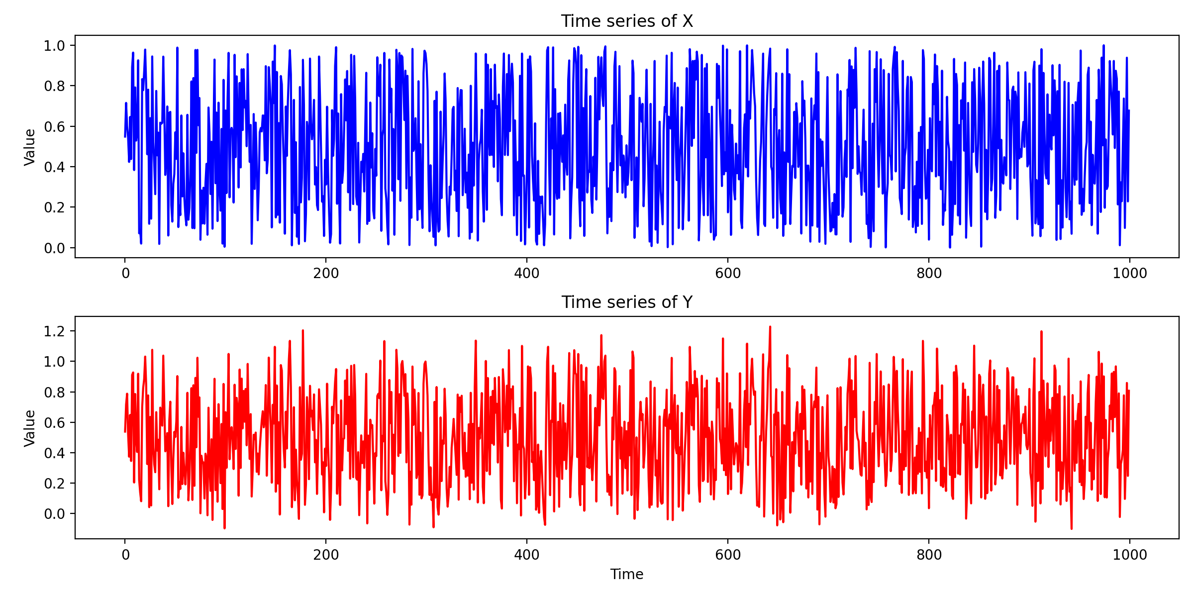The two generated time series.

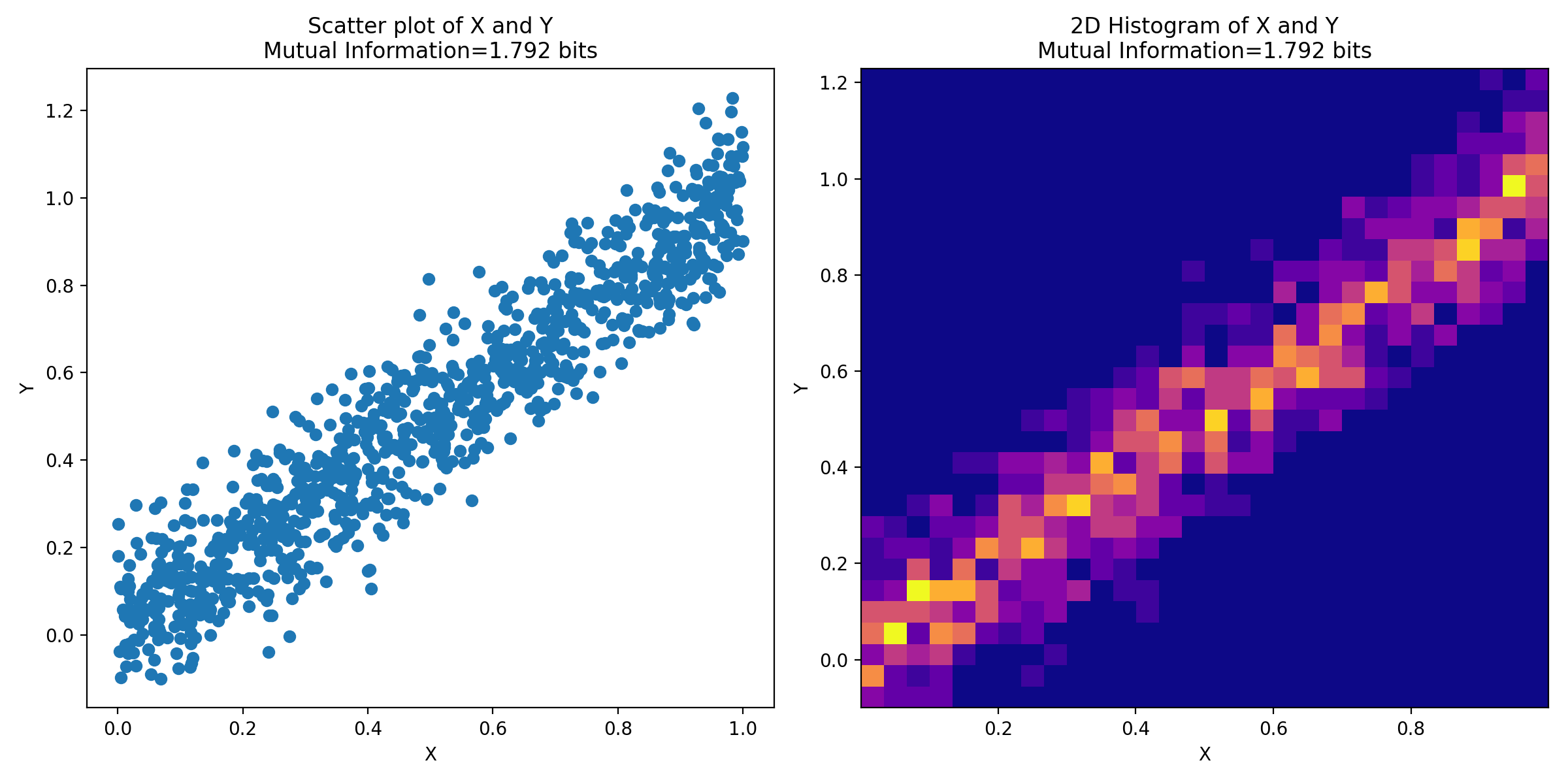2D histogram and scatter plot, visualizing the joint distribution of the two time series.

The 2D histogram and scatter plot are used to visualize the joint distribution of the two variables, allowing us to have a visual interpretation of the dependence between them. The 2D histogram groups pairs of $(X,Y)$ into bins and the color indicates the number of pairs in each bin. It is particularly useful when we have many data points, as it can provide a clearer visualization of the density of points. Areas of the plot with a high density of points (darker color) indicate combinations of $X$ and $Y$ that occur more frequently. The scatter plot, on the other hand, plots each pair of $(X, Y)$ as a single point in two-dimensional space, allowing us to observe the raw relationship between $X$ and $Y$. Each point represents an instance of time in the time series.

A mutual information value of 1.79 bits indicates that the two time series are highly dependent on each other. This is also evident from the 2D histogram and scatter plot, where we can see that the two time series are highly correlated. The scatter plot shows a clear linear relationship between $X$ and $Y$, while the 2D histogram shows a high density of points along the diagonal, indicating that the two time series are highly correlated.

Mutual information vs. correlation analysis

After the discussion of the example above and from what we have learned so far, one might wonder: Are mutual information and correlation analysis to some extent interchangeable? The Answer is: No, they are not.

While both mutual information and correlation measures capture dependencies between variables, they are inherently different. Correlation coefficients only capture linear relationships between variables, while mutual information can capture any kind of statistical dependence, including non-linear ones. However, one should be careful with MI since it doesn’t distinguish between direct and indirect effects. Therefore, while MI provides a more general measure of association between two variables, it does not necessarily serve as a direct substitute for correlation analysis.

Conclusion

Mutual Information (MI) and its correlation with Information Entropy provide profound insights into the intricate statistical dependencies between variables. This fundamental knowledge forms the backbone of various techniques employed across disciplines, from machine learning to neuroscience. While MI offers a robust measure capable of capturing both linear and non-linear associations, it’s essential to acknowledge its limitations, particularly its inability to differentiate between direct and indirect relationships. Therefore, while MI offers a comprehensive measure of association, it cannot completely replace correlation analysis, which holds its unique strengths, especially in analyzing linear relationships. Hence, the choice between using MI or correlation should be context-dependent, guided by the specifics of the problem at hand.

If you have any questions or suggestions, feel free to leave a comment below or reach out to me on Mastodonꜛ.

The code used in this post is also available in this GitHub repositoryꜛ.