Enable interactive plots and other plot modes in Jupyter notebooks

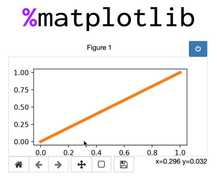
The so-called magic command %matplotlib enables us to control the behavior of plots in Jupyter notebook.

Magic commands are specific Python commands provided by the IPythonꜛ kernel. They serve as shortcuts of common operations for solving frequent problems in data analysis. There are two different types of magic commands:

• line magics, prefixed by %. They run over on a single line of code.
• cell magics, by %%. They run over an entire cell.

For instance, the %who and the %whos commands list all variables that are defined in the current notebook session:

a = 9
b = 99.0
c = 999
%whos

    Variable                        Type        Data/Info
    -----------------------------------------------------
    a                               int         9
    b                               float       99.0
    c                               int         999

The %%time command helps to track the total execution time for the code of one cell:

%%time
x=0
for i in range(10000):
    x+=i**2

    CPU times: user 4.16 ms, sys: 13 µs, total: 4.18 ms
    Wall time: 4.3 ms

To get a list of all currently available magic commands, execute %lsmagic:

%lsmagic

    Available line magics:
    %alias  %alias_magic  %autoawait  %autocall  %automagic  %autosave  %bookmark  %cat  
    %cd  %clear  %colors  %conda  %config  %connect_info  %cp  %debug  %dhist  %dirs 
    %doctest_mode  %ed  %edit  %env  %gui  %hist  %history  %killbgscripts  %ldir  
    %less  %lf  %lk  %ll  %load  %load_ext  %loadpy  %logoff  %logon  %logstart  %logstate 
    %logstop  %ls  %lsmagic  %lx  %macro  %magic  %man  %matplotlib  %mkdir  %more  %mv 
    %notebook  %page  %pastebin  %pdb  %pdef  %pdoc  %pfile  %pinfo  %pinfo2  %pip  %popd 
    %pprint  %precision  %prun  %psearch  %psource  %pushd  %pwd  %pycat  %pylab  
    %qtconsole  %quickref  %recall  %rehashx  %reload_ext  %rep  %rerun  %reset  
    %reset_selective  %rm  %rmdir  %run  %save  %sc  %set_env  %store  %sx  %system 
    %tb  %time  %timeit  %unalias  %unload_ext  %who  %who_ls  %whos  %xdel  %xmode

    Available cell magics:
    %%!  %%HTML  %%SVG  %%bash  %%capture  %%debug  %%file  %%html  %%javascript  %%js  
    %%latex  %%markdown  %%perl  %%prun  %%pypy  %%python  %%python2  %%python3  %%ruby  
    %%script  %%sh  %%svg  %%sx  %%system  %%time  %%timeit  %%writefile

A reference of all magic commands is available on the IPython documentation websiteꜛ.

Magic commands to control matplotlib plots

With the %matplotlibꜛ magic command we can control the currently activated GUI backend for matplotlib. The %matplotlib --list lists of all available backends:

%matplotlib --list

    Available matplotlib backends: ['tk', 'gtk', 'gtk3', 'gtk4', 'wx', 'qt4', 'qt5', 'qt6', 
    'qt', 'osx', 'nbagg', 'webagg', 'notebook', 'agg', 'svg', 'pdf', 'ps', 'inline', 
    'ipympl', 'widget']

For reproducibility, the following examples were created with the following dependencies:

conda create -n JupyterLab -y python=3.9
conda activate JupyterLab
conda install -y matplotlib numpy ipykernel ipympl jupyter notebook ipython

All examples are also available in this Jupyter notebook:

Get interactive plots with %matplotlib notebook

The default mode of matplotlib plots in Jupyter notebooks is the static inline mode. To change that mode and get interactive plots, simply add the magic command %matplotlib notebook to your notebook once:

%matplotlib notebook
import matplotlib.pyplot as plt

Once executed, all your plots will be interactive, i.e., you can zoom in and out, navigate in the plot, or save it to disk. And you can still apply changes to it, even if these changes are applied in a different cell. For example, execute the following two cells one after another:

# generate the plot figure and add the first plot:
fig=plt.figure(1, figsize=(4,2))
plt.clf()
plt.plot([[0, 0], [1,1]], linewidth=4, label='random diagonal')
plt.show ()

# in a different cell, add another plot to the same figure:
plt.plot([[1, 1], [0,0]], linewidth=2, label='random diagonal')

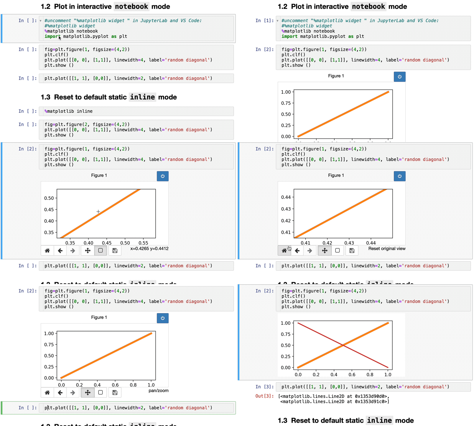
To stop the interactive mode for a specific plot figure, just click the blue power button in the upper right corner.

JupyterLab and VS Code
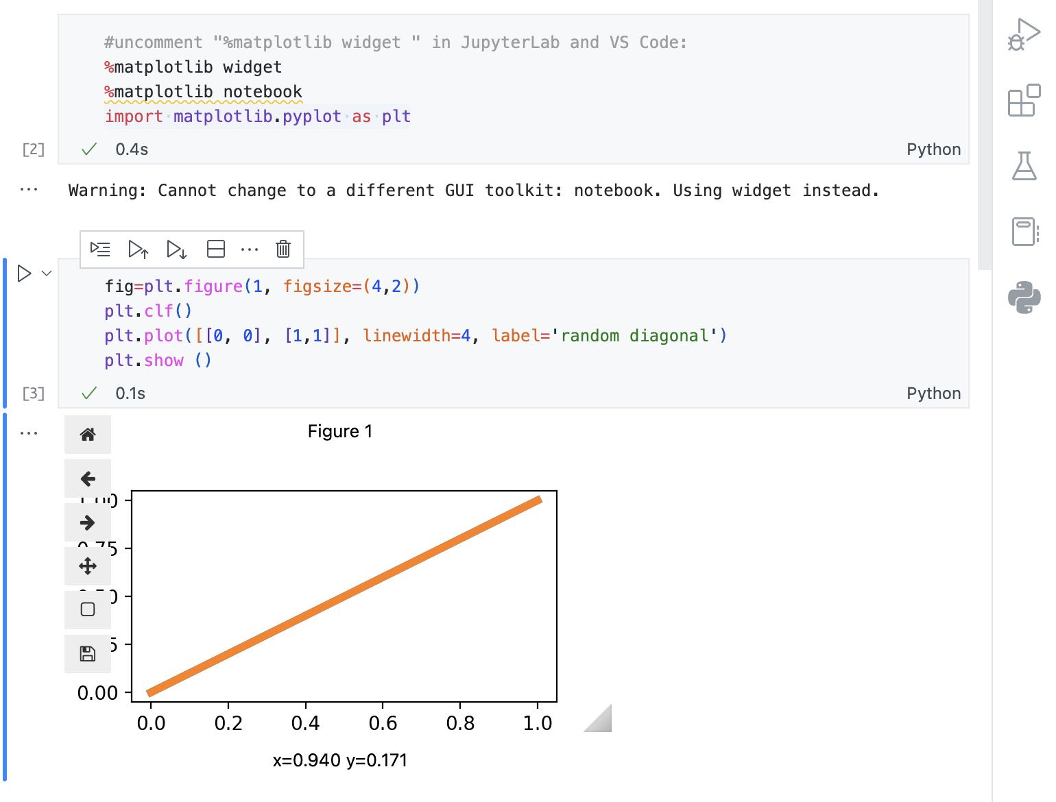
In JupyterLab and VS Code, we have to use the %matplotlib widget command instead, otherwise the interactive plots won’t show up:

%matplotlib widget
import matplotlib.pyplot as plt

The plots then look a little different, and we don’t have that blue shutdown button. But apart from that, we can interact with the plot as described above:

Reset to the default static mode with %matplotlib inline

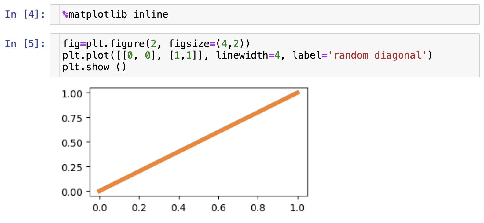
To reset to the default static mode, simply execute the %matplotlib inline command:

%matplotlib inline

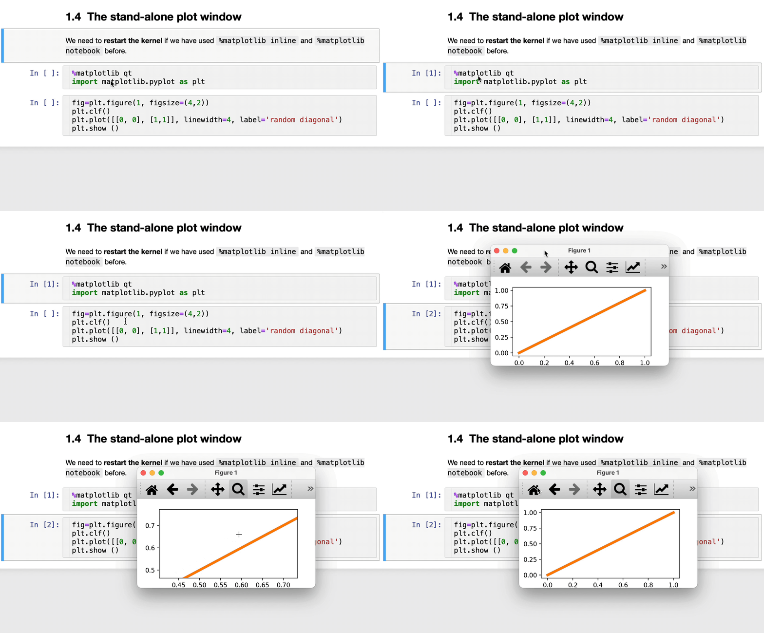
Activate stand-alone plot windows with %matplotlib qt

To get interactive stand-alone plot windows, we can use the %matplotlib qt magic command. However, if we have run the %matplotlib notebook command before, we have to restart the Jupyter kernel first.

%matplotlib qt
import matplotlib.pyplot as plt