The Weierstrass function and the beauty of fractals

Fractals are captivating mathematical objects that exhibit intricate patterns and self-similarity at various scales. In this post, we explore the elegance and significance of the Weierstrass function, its relation to fractals and fractal geometry, and discuss other notable fractals such as the Takagi function, the Mandelbrot set, Julia set, Koch curve (Koch snowflake), and the Sierpinski triangle. Through this journey, we will discover the fascinating world of fractal geometry and its beautiful and profound impact.

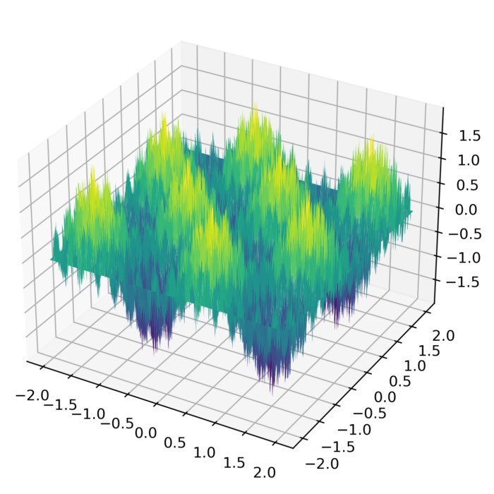
Weierstrass function: A continuous yet nowhere differentiable phenomenon

The Weierstrass function, named after mathematician Karl Weierstrass, serves as an exemplary instance of a continuous but nowhere differentiable function. It is defined as follows:

\[f(x) = \sum_{n=0}^{\infty} a^n \cos(b^n \pi x)\]

where $a$ and $b$ are parameters such that $0 \lt a \lt 1$ and $b$ is an odd integer.

The Weierstrass function is significant in mathematics because it provides an example of a function that challenges our intuition about differentiability. Unlike many familiar functions, such as polynomials or trigonometric functions, the Weierstrass function is continuous at every point but does not possess a derivative anywhere. In other words, its graph is incredibly rough and jagged, exhibiting intricate self-similarity at different scales.

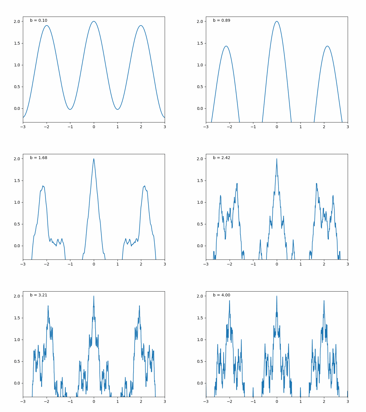The Weierstrass function in 1D. The function is continuous but nowhere differentiable. The Python code used to generate this animation is shown below and also available in the GitHub repository linked at the end of this post.

import numpy as np
import matplotlib.pyplot as plt
from matplotlib.animation import FuncAnimation, PillowWriter

# setting the ranges for calculation: 
b_start = -3
b_stop = 3
steps = 1000

# b for x axis. Here you can change start and stop points:
b = np.arange(b_start, b_stop, ((b_stop-b_start)/steps))

# defining the weierstrass function:
def weierstrass(x, Nvar, b):
    ws = np.zeros(steps)
    for n in range(0, Nvar):
        ws = ws + np.cos(b**n*np.pi*x)/2**n
    return ws

# plot/animate:
fig, ax = plt.subplots()
ax.set_xlim(b_start, b_stop)
line, = ax.plot(b, weierstrass(b, 500, 0.1))
ax.annotate(f'b = {0.1:.2f}', (0.05, 0.95), xycoords='axes fraction')

def update(b):
    line.set_ydata(weierstrass(b, 500, b))
    ax.texts[0].set_text(f'b = {b:.2f}')
    return line,

ani = FuncAnimation(fig, update, frames=np.linspace(0.1, 4, 100), interval=50)
writer = PillowWriter(fps=15)
ani.save('weierstrass_function.gif', writer=writer)
plt.show()

The function has found applications in areas such as signal processing, image compression, and data encryption. Its irregular and self-similar nature can be exploited in various algorithms to generate pseudorandom numbers or create complex patterns.

Furthermore, one of the many applications of the Weierstrass function is in the field of fractal geometry. Fractals are complex geometric shapes that exhibit self-similarity and have fractional dimensions. The Weierstrass function serves as an example of a fractal curve due to its self-similar nature. This function demonstrates a fractal-like nature due to the infinite summation of cosine functions with varying frequencies and amplitudes. Each term contributes to the complexity and self-similarity of the function, resulting in the lack of differentiability throughout its domain.

However, the Weierstrass function is not commonly used to generate fractal shapes in the same way as other fractal generation techniques such as the Mandelbrot set or the Koch snowflake. But we can use the Weierstrass function to generate a fractal landscape by stacking multiple plots of the function with varying amplitudes and frequencies. Here is an example generate with the Python code shown below:

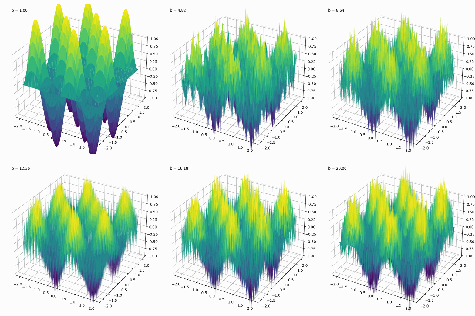A fractal landscape generated by stacking multiple plots of the Weierstrass function with varying amplitudes and frequencies. The Python code used to generate this animation is shown below.

# setting the ranges for calculation:
b_start = -2
b_stop = 2
steps = 1000

# set b for x axis. Here you can change start and stop points:
x = np.linspace(b_start, b_stop, steps)
X, Y = np.meshgrid(x, x)

# defining the weierstrass function:
def weierstrass(x, y, Nvar, b):
    Z = np.zeros((steps, steps))
    for n in range(0, Nvar):
        Z += (0.5**n) * np.sin((b**n) * (np.pi * x)) * np.sin((b**n) * (np.pi * y))
    return Z

# plot/animate:
fig = plt.figure(figsize=(6, 6))
ax = fig.add_subplot(111, projection='3d')
ax.set_zlim(-1, 1)
surf = ax.plot_surface(X, Y, weierstrass(X, Y, 10, 1))
text = ax.text2D(0.05, 0.95, f"b = {1}", transform=ax.transAxes)

def update(b):
    ax.clear()
    ax.set_zlim(-1, 1)
    surf = ax.plot_surface(X, Y, weierstrass(X, Y, 10, b), cmap='viridis')
    text = ax.text2D(0.05, 0.95, f"b = {b:.2f}", transform=ax.transAxes)
    plt.tight_layout()
    return surf,

ani = FuncAnimation(fig, update, frames=np.linspace(1, 20, 200), interval=100)
writer = PillowWriter(fps=10)
ani.save('weierstrass_fractal.gif', writer=writer)
plt.show()

Fractal landscapes, also known as height maps or terrain models, have many potential use cases in fields such as computer graphics, video game design, and geology. They can be used to generate realistic and visually appealing terrain for virtual environments, animations, and simulations. For example, in computer graphics and video game design, fractal landscapes can be used to create realistic terrain for outdoor scenes and environments. The self-similar nature of fractals allows for the generation of detailed landscapes at multiple levels of scale, from large mountain ranges to small rocks and pebbles. In geology, fractal landscapes can be used to model and simulate natural terrain formations and processes such as erosion and sedimentation. This can help researchers better understand the underlying mechanisms behind these processes and make more accurate predictions about how landscapes will change over time.

Fractal functions: Weierstrass and Takagi as examples

The Weierstrass function is part of a broader class known as fractal functions, which exhibit self-similarity and intricate patterns. Another notable function in this class is the Takagi function, also referred to as the Takagi-Landsberg function or the Blancmange curve. It is defined as:

\[T(x) = \sum_{n=0}^{\infty} \frac{\phi(2^n x)}{2^n}\]

where $\phi(x)$ represents the distance from $x$ to the nearest integer. Like the Weierstrass function, the Takagi function is continuous but nowhere differentiable, showcasing its fractal-like properties and self-similarity.

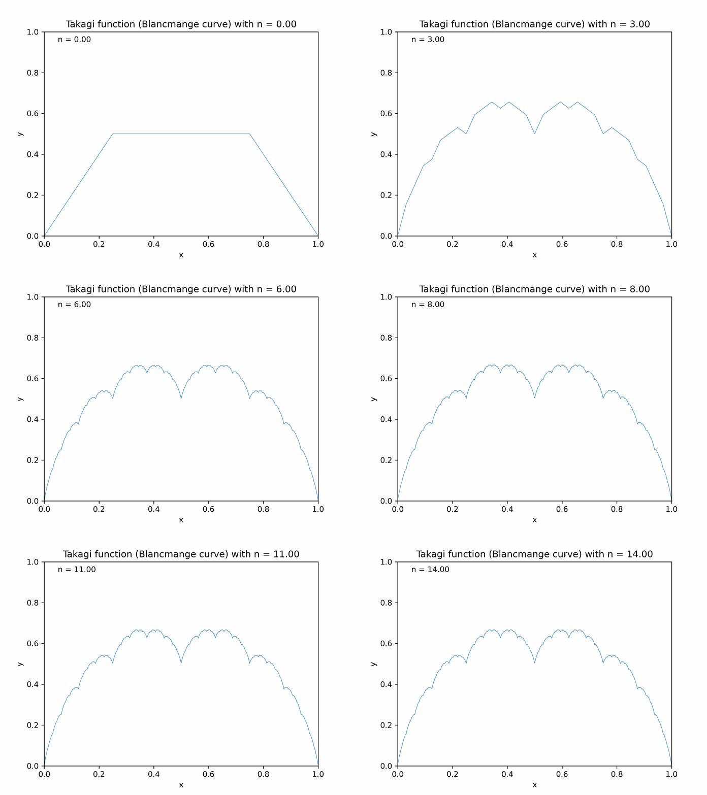Animation of the Takagi function (Blancmange curve) with increasing $n$, generated with the Python code is shown below.

import numpy as np
import matplotlib.pyplot as plt
from matplotlib.animation import FuncAnimation

def phi(x):
    return np.abs(x - np.floor(x + 0.5)).astype(float)

def takagi(x, n):
    result = np.zeros_like(x, dtype=float)
    for i in range(n + 1):
        result = np.add(result, phi(2**i * x) / 2**i, out=result, casting="unsafe")
    return result

fig, ax = plt.subplots()
ax.set_xlim(0, 1)
ax.set_ylim(0, 1)
line, = ax.plot([], [], lw=0.5)
ax.annotate(f'n = {0.0:.2f}', (0.05, 0.95), xycoords='axes fraction')

def init():
    line.set_data([], [])
    return line,

def update(frame):
    x = np.linspace(0, 1, 1000)
    y = takagi(x, frame + 1)
    line.set_data(x, y)
    # Annotate current n:
    ax.texts[0].set_text(f'n = {frame:.2f}')
    ax.set_title(f'Takagi function (Blancmange curve) with n = {frame:.2f}')
    ax.set_xlabel('x')
    ax.set_ylabel('y')
    return line

# Set up the animation and save as GIF:
anim = FuncAnimation(fig, update, frames=15, init_func=init, blit=True)
anim.save('takagi_animation.gif', writer='pillow', dpi=300)
plt.show()

Mandelbrot set: Exploring infinite complexity

The Mandelbrot set, denoted by $M$, is a remarkable fractal formed by iterating the complex quadratic polynomial $f_c(z) = z^2 + c$. It can be defined as the set of complex numbers $c$ for which the iteration remains bounded. Mathematically, it is represented as:

\[M = \{c \in \mathbb{C} : z_{n+1} = z_n^2 + c, \text{ remains bounded}\}\]

The Mandelbrot set reveals an infinite variety of intricate patterns when visualized, exhibiting self-similarity and complexity at all levels of magnification.

Animation of the Mandelbrot set with increasing $n$. The Python code to generate this animation is taken from the matplotlib.org documentationꜛ.

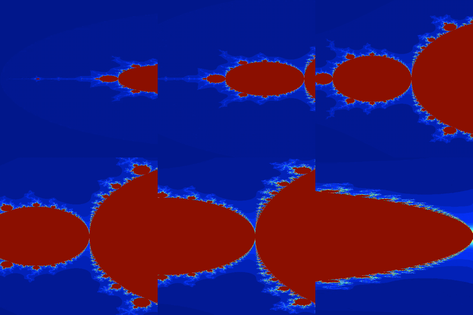Another animation of the Mandelbrot set with zoom-effect. The Python code to generate this animation is shown below.

import numpy as np
import matplotlib.pyplot as plt
import matplotlib.animation as animation
import imageio
import os

def mandelbrot(x, y, threshold):
    """Calculates whether the number c = x + i*y belongs to the 
    Mandelbrot set. In order to belong, the sequence z[i + 1] = z[i]**2 + c
    must not diverge after 'threshold' number of steps. The sequence diverges
    if the absolute value of z[i+1] is greater than 4.
    
    :param float x: the x component of the initial complex number
    :param float y: the y component of the initial complex number
    :param int threshold: the number of iterations to considered it converged
    """
    # initial conditions:
    c = complex(x, y)
    z = complex(0, 0)
    
    for i in range(threshold):
        z = z**2 + c
        if abs(z) > 4.:  # it diverged
            return i
        
    return threshold - 1  # it didn't diverge

x_start, y_start = -2, -1.5  # an interesting region starts here
width, height = 3, 3  # for 3 units up and right
density_per_unit = 250  # how many pixles per unit

# real and imaginary axis:
re = np.linspace(x_start, x_start + width, width * density_per_unit )
im = np.linspace(y_start, y_start + height, height * density_per_unit)

fig = plt.figure(figsize=(10, 10))  # instantiate a figure to draw
ax = plt.axes()  # create an axes object

def animate(i):
    ax.clear()  # clear axes object
    ax.set_xticks([], [])  # clear x-axis ticks
    ax.set_yticks([], [])  # clear y-axis ticks
    
    X = np.empty((len(re), len(im)))  # re-initialize the array-like image
    threshold = round(1.15**(i + 1))  # calculate the current threshold
    
    # iterations for the current threshold:
    for i in range(len(re)):
        for j in range(len(im)):
            X[i, j] = mandelbrot(re[i], im[j], threshold)
    
    # associate colors to the iterations with an iterpolation:
    img = ax.imshow(X.T, interpolation="bicubic", cmap='magma')
    plt.tight_layout()
    return [img]
 
anim = animation.FuncAnimation(fig, animate, frames=45, interval=120, blit=True)
anim.save('mandelbrot.gif',writer='imagemagick')

and

# %% MANDELBROT SET ANIMATION (FROM SCRATCH)

def mandelbrot(c, max_iter):
    z = c
    for n in range(max_iter):
        if abs(z) > 2:
            return n
        z = z*z + c
    return max_iter

def mandelbrot_set(xmin,xmax,ymin,ymax,width,height,max_iter):
    r1 = np.linspace(xmin, xmax, width)
    r2 = np.linspace(ymin, ymax, height)
    return (r1,r2,np.array([[mandelbrot(complex(r, i),max_iter) for r in r1] for i in r2]))

images = []
n_frames = 82

for i in range(n_frames):
    dpi = 120
    img_width = 800
    img_height = 800
    fig = plt.figure(figsize=(img_width/dpi, img_height/dpi), dpi=dpi)
    ax = fig.add_axes([0, 0, 1, 1], frameon=False, aspect=1)

    # Adjust the coordinates for zooming effect
    if i < 36:
        xmin = -2.0+0.02*i
        xmax = -1.0+0.02*i
        ymin = -1.5+0.02*i
        ymax = 1.5-0.02*i
    else:
        xmin = (-2.0+0.02*35) + (0.01*(i-35))
        xmax = (-1.0+0.02*35) - (0.01*(i-35))
        ymin = (-1.5+0.02*35) + (0.01*(i-35))
        ymax = (1.5-0.02*35) - (0.01*(i-35))

    pixels = mandelbrot_set(xmin, xmax, ymin, ymax, 800, 800, 256)
    ax.imshow(pixels[2], origin="lower", cmap="jet")
    
    plt.xticks([])
    plt.yticks([])
    plt.tight_layout()

    # Check if the frames directory exists and create it if necessary:
    if not os.path.exists("mandelbrot_frames"):
        os.makedirs("mandelbrot_frames")
    plt.savefig("mandelbrot_frames/frame_{}.png".format(i))
    images.append(imageio.imread("mandelbrot_frames/frame_{}.png".format(i)))

# Ensure you have a directory called 'images/images' or adjust the path as needed
imageio.mimsave('images/mandelbrot_zoom.gif', images[:82])

Julia Set: Unveiling fractal beauty

The Julia set, denoted by $J_c$, is closely related to the Mandelbrot set. It represents the set of complex numbers $z$ for which the iteration $f_c(z) = z^2 + c$ remains bounded. Each $c$ value gives rise to a unique Julia set with its own fascinating fractal pattern. The Julia set can be mathematically defined as:

\[J_c = \{z \in \mathbb{C} : f_c^n(z) \text{ does not tend to infinity}\}\]

where $f_c^n(z)$ represents the $n$-th iteration of $f_c(z)$.

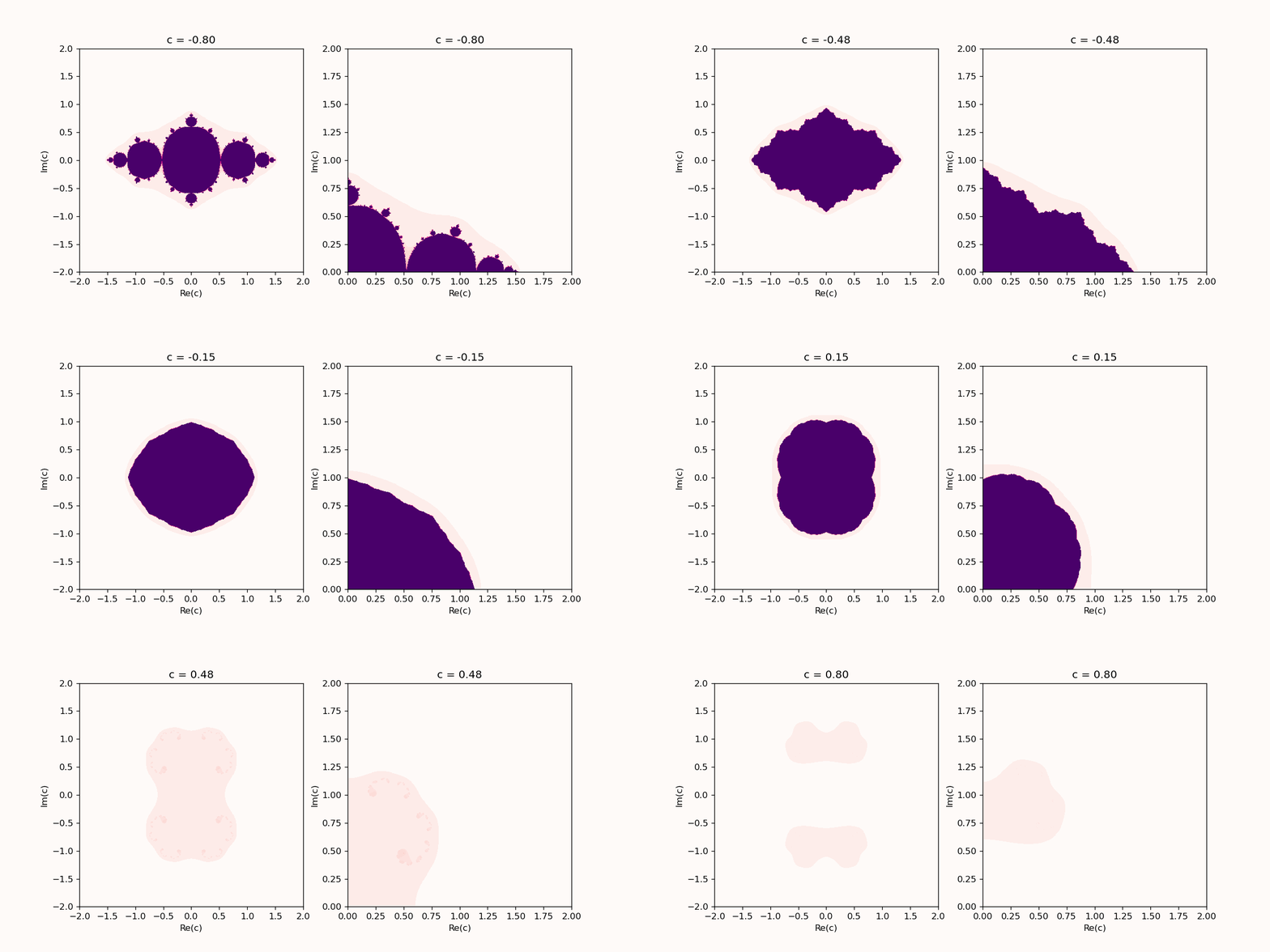Animation of the Julia set with increasing $n$. The left panel shows a zoom on the upper right quadrant of the left panel. The Python code to generate this animation is shown below.

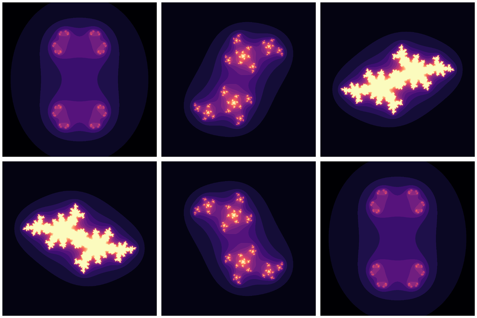Another animation of the Julia set. The Python code (“JULIA SET 2”) to generate this animation is taken from the matplotlib.org documentationꜛ.

import numpy as np
import matplotlib.pyplot as plt
from matplotlib.animation import FuncAnimation

# %% JULIA SET 1:
def julia_set(c, width, height, x_min, x_max, y_min, y_max, max_iter):
    x = np.linspace(x_min, x_max, width)
    y = np.linspace(y_min, y_max, height)
    X, Y = np.meshgrid(x, y)
    Z = X + 1j * Y

    img = np.zeros_like(Z, dtype=int)

    for i in range(max_iter):
        mask = np.abs(Z) < 4
        Z[mask] = Z[mask] ** 2 + c
        img += mask

    return img

# set up the figure and subplots:
fig, (ax1, ax2) = plt.subplots(1, 2, figsize=(10, 5))

# common parameters:
width, height = 400, 400
x_min, x_max = -2.0, 2.0
y_min, y_max = -2.0, 2.0
c_values = np.linspace(-0.8, 0.8, 100)  # different values of the parameter 'c'
max_iter = 100

# plot 1 - full Julia set:
img1 = ax1.imshow(julia_set(c_values[0], width, height, x_min, x_max, y_min, y_max, max_iter),
                  cmap='RdPu', extent=(x_min, x_max, y_min, y_max), origin='lower')
ax1.set_title('Julia Set (Full)')
ax1.set_xlabel('Re(c)')
ax1.set_ylabel('Im(c)')

# plot 2 - zoomed-in Julia set:
zoom_factor = 0.5
zoom_x_min = x_max - (x_max - x_min) * zoom_factor
zoom_x_max = x_max
zoom_y_min = y_max - (y_max - y_min) * zoom_factor
zoom_y_max = y_max
img2 = ax2.imshow(julia_set(c_values[0], width, height, zoom_x_min, zoom_x_max, zoom_y_min, zoom_y_max, max_iter),
                  cmap='RdPu', extent=(zoom_x_min, zoom_x_max, zoom_y_min, zoom_y_max), origin='lower')
ax2.set_title('Julia Set (Zoomed)')
ax2.set_xlabel('Re(c)')
ax2.set_ylabel('Im(c)')

# update function:
def update(frame):
    # update plot 1 - full Julia set:
    img1.set_array(julia_set(c_values[frame], width, height, x_min, x_max, y_min, y_max, max_iter))
    ax1.set_title(f"c = {c_values[frame]:.2f}")

    # update plot 2 - zoomed-in Julia set:
    img2.set_array(julia_set(c_values[frame], width, height, zoom_x_min, zoom_x_max, zoom_y_min, zoom_y_max, max_iter))
    ax2.set_title(f"c = {c_values[frame]:.2f}")

# create and save the animation:
anim = FuncAnimation(fig, update, frames=len(c_values), interval=100)
anim.save('julia_set_animation.gif', writer='pillow', dpi=120)
plt.show()

and

# %% JULIA SET 2:
# define parameters:
x_start, y_start = -2, -2  # an interesting region starts here
width, height = 4, 4  # for 4 units up and right
density_per_unit = 200  # how many pixles per unit

# real and imaginary axis:
re = np.linspace(x_start, x_start + width, width * density_per_unit )
im = np.linspace(y_start, y_start + height, height * density_per_unit)

threshold = 20  # max allowed iterations
frames = 100  # number of frames in the animation

# we represent c as c = r*cos(a) + i*r*sin(a) = r*e^{i*a}:
r = 0.7885
a = np.linspace(0, 2*np.pi, frames)

fig = plt.figure(figsize=(10, 10))  # instantiate a figure to draw
ax = plt.axes()  # create an axes object

def julia_quadratic(zx, zy, cx, cy, threshold):
    """Calculates whether the number z[0] = zx + i*zy with a constant c = x + i*y
    belongs to the Julia set. In order to belong, the sequence 
    z[i + 1] = z[i]**2 + c, must not diverge after 'threshold' number of steps.
    The sequence diverges if the absolute value of z[i+1] is greater than 4.
    
    :param float zx: the x component of z[0]
    :param float zy: the y component of z[0]
    :param float cx: the x component of the constant c
    :param float cy: the y component of the constant c
    :param int threshold: the number of iterations to considered it converged
    """
    # initial conditions
    z = complex(zx, zy)
    c = complex(cx, cy)
    
    for i in range(threshold):
        z = z**2 + c
        if abs(z) > 4.:  # it diverged
            return i
        
    return threshold - 1  # it didn't diverge

def animate(i):
    ax.clear()  # clear axes object
    ax.set_xticks([], [])  # clear x-axis ticks
    ax.set_yticks([], [])  # clear y-axis ticks
    
    X = np.empty((len(re), len(im)))  # the initial array-like image
    cx, cy = r * np.cos(a[i]), r * np.sin(a[i])  # the initial c number
    
    # iterations for the given threshold
    for i in range(len(re)):
        for j in range(len(im)):
            X[i, j] = julia_quadratic(re[i], im[j], cx, cy, threshold)
    
    img = ax.imshow(X.T, interpolation="bicubic", cmap='magma')
    plt.tight_layout()
    return [img]

anim = animation.FuncAnimation(fig, animate, frames=frames, interval=50, blit=True)
anim.save('julia_set_animation_2.gif', writer='imagemagick')

Koch snowflake: Beauty in self-similarity:

The Koch curve, often referred to as the Koch snowflake, is a fractal constructed by iteratively replacing line segments with a specific pattern. Starting with a simple equilateral triangle, each line segment is divided into three equal parts, and an equilateral triangle is constructed on the middle segment. This process is repeated infinitely, resulting in a snowflake-like fractal shape. Mathematically, the Koch curve can be defined using recursive formulas.

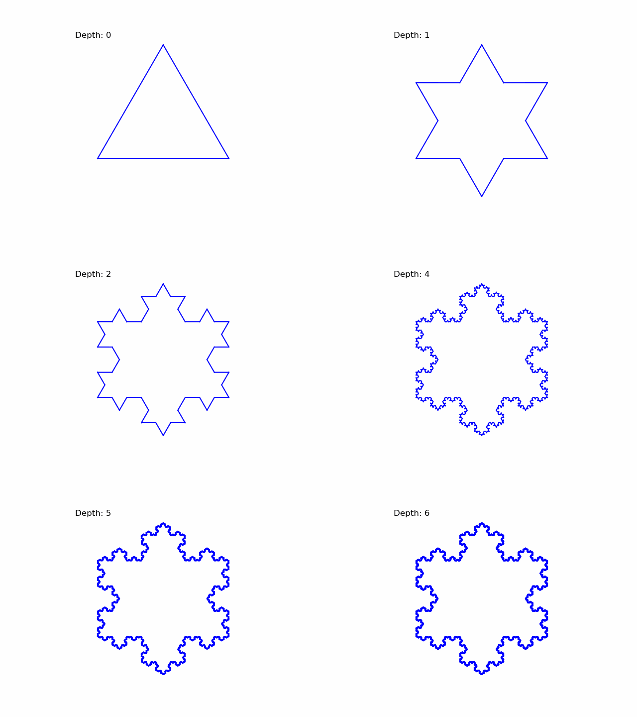Animation of the Koch snowflake set with increasing depth. The Python code to generate this animation is shown below.

The same animation as before, but with changing colors. This animation was actually an accident I wanted to change the color of the snowflake with each recursion level, but I messed it up and also the color of the line segments is now changing. However, I thought it looked pretty cool, so I decided to keep it. The Python code to generate this animation is also shown below.

import numpy as np
import matplotlib.pyplot as plt
from matplotlib.animation import FuncAnimation
import random

# %% KOCH SNOWFLAKE ANIMATION
def koch_snowflake(ax, p1, p2, depth=0):
    if depth == 0:
        ax.plot([p1[0], p2[0]], [p1[1], p2[1]], color='b')
    else:
        dx = p2[0] - p1[0]
        dy = p2[1] - p1[1]
        length = np.sqrt(dx**2 + dy**2)
        unit = length / 3.0
        angle = np.arctan2(dy, dx)

        p1_new = p1
        p2_new = [p1[0] + np.cos(angle) * unit, p1[1] + np.sin(angle) * unit]
        p3_new = [p2_new[0] + np.cos(angle - np.pi / 3) * unit, p2_new[1] + np.sin(angle - np.pi / 3) * unit]
        p4_new = [p1[0] + np.cos(angle) * 2 * unit, p1[1] + np.sin(angle) * 2 * unit]

        koch_snowflake(ax, p1_new, p2_new, depth - 1)
        koch_snowflake(ax, p2_new, p3_new, depth - 1)
        koch_snowflake(ax, p3_new, p4_new, depth - 1)
        koch_snowflake(ax, p4_new, p2, depth - 1)

fig, ax = plt.subplots()
ax.set_aspect('equal')
ax.axis('off')

# initial points of the Koch snowflake:
p1 = [-0.5, -0.288]
p2 = [0.5, -0.288]
p3 = [0.0, 0.577]

depth = 5  # Set the desired depth of recursion

def update(frame):
    ax.clear()
    ax.set_aspect('equal')
    ax.axis('off')

    # calculate the new points for the current frame:
    new_p1 = p1
    new_p2 = p2
    new_p3 = p3

    # adjust the depth for each frame:
    current_depth = int(depth * (frame + 1) / 100.0)

    # Generate the Koch snowflake
    koch_snowflake(ax, new_p1, new_p2, current_depth)
    koch_snowflake(ax, new_p2, new_p3, current_depth)
    koch_snowflake(ax, new_p3, new_p1, current_depth)

    # set the plot limits:
    ax.set_xlim([-0.7, 0.7])
    ax.set_ylim([-0.7, 0.7])

    # annotate the depth in the plot:
    ax.text(0.02, 0.95, 'Depth: {}'.format(current_depth), transform=ax.transAxes, color='black', fontsize=12)

anim = FuncAnimation(fig, update, frames=120, interval=100)
anim.save('koch_snowflake_animation.gif', writer='pillow', fps=60)
plt.show()

and

# %% KOCH SNOWFLAKE ANIMATION W/ CHANGING COLORS
def koch_snowflake(ax, p1, p2, depth=0, color='b'):
    if depth == 0:
        ax.plot([p1[0], p2[0]], [p1[1], p2[1]], color=color)
    else:
        dx = p2[0] - p1[0]
        dy = p2[1] - p1[1]
        length = np.sqrt(dx**2 + dy**2)
        unit = length / 3.0
        angle = np.arctan2(dy, dx)

        p1_new = p1
        p2_new = [p1[0] + np.cos(angle) * unit, p1[1] + np.sin(angle) * unit]
        p3_new = [p2_new[0] + np.cos(angle - np.pi / 3) * unit, p2_new[1] + np.sin(angle - np.pi / 3) * unit]
        p4_new = [p1[0] + np.cos(angle) * 2 * unit, p1[1] + np.sin(angle) * 2 * unit]

        # generate a random color for each recursion level:
        new_color = '#' + ''.join(random.choices('0123456789ABCDEF', k=6))

        koch_snowflake(ax, p1_new, p2_new, depth - 1, new_color)
        koch_snowflake(ax, p2_new, p3_new, depth - 1, new_color)
        koch_snowflake(ax, p3_new, p4_new, depth - 1, new_color)
        koch_snowflake(ax, p4_new, p2, depth - 1, new_color)

fig, ax = plt.subplots()
ax.set_aspect('equal')
ax.axis('off')

# initial points of the Koch snowflake:
p1 = [-0.5, -0.288]
p2 = [0.5, -0.288]
p3 = [0.0, 0.577]

depth = 5  # set the desired depth of recursion

def update(frame):
    ax.clear()
    ax.set_aspect('equal')
    ax.axis('off')

    # calculate the new points for the current frame:
    new_p1 = p1
    new_p2 = p2
    new_p3 = p3

    # adjust the depth for each frame:
    current_depth = int(depth * (frame + 1) / 100.0)

    # generate the Koch snowflake:
    koch_snowflake(ax, new_p1, new_p2, current_depth)
    koch_snowflake(ax, new_p2, new_p3, current_depth)
    koch_snowflake(ax, new_p3, new_p1, current_depth)

    # set the plot limits:
    ax.set_xlim([-0.7, 0.7])
    ax.set_ylim([-0.7, 0.7])

    # annotate the depth in the plot:
    ax.text(0.02, 0.95, 'Depth: {}'.format(current_depth), transform=ax.transAxes, color='black', fontsize=12)

anim = FuncAnimation(fig, update, frames=100, interval=100)
anim.save('koch_snowflake_animation_color.gif', writer='pillow', fps=60)
plt.show()

Sierpinski triangle: Intricacy in triangular form

The Sierpinski triangle is a captivating fractal composed of an infinite number of smaller triangles arranged in a specific pattern. It is created by iteratively removing the central triangle from each larger triangle, resulting in a fractal with self-similarity and intricate detail. The Sierpinski triangle can be defined recursively using graphical techniques or mathematically through iterative algorithms.

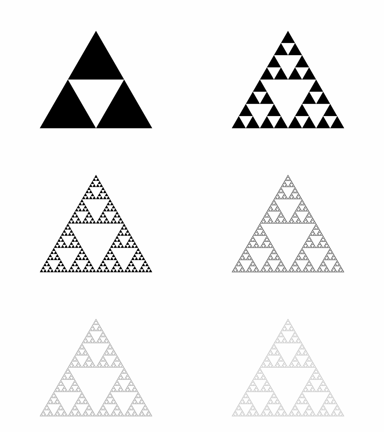Animation of the Sierpinski triangle set with increasing depth. The Python code to generate this animation is shown below.

import numpy as np
import matplotlib.pyplot as plt
from matplotlib.animation import FuncAnimation
# %% SIERPINSKI TRIANGLE
def sierpinski_triangle(ax, p1, p2, p3, depth=0):
    if depth == 0:
        ax.fill([p1[0], p2[0], p3[0]], [p1[1], p2[1], p3[1]], 'k')
    else:
        p12 = (p1 + p2) / 2
        p23 = (p2 + p3) / 2
        p31 = (p3 + p1) / 2
        
        sierpinski_triangle(ax, p1, p12, p31, depth - 1)
        sierpinski_triangle(ax, p12, p2, p23, depth - 1)
        sierpinski_triangle(ax, p31, p23, p3, depth - 1)

def update(frame):
    ax.clear()
    ax.set_aspect('equal')
    ax.axis('off')
    
    depth = frame + 1
    sierpinski_triangle(ax, p1, p2, p3, depth)
    
    ax.set_xlim(-0.1, 1.1)
    ax.set_ylim(-0.1, 1.1)
    plt.tight_layout()

# initialize the plot:
fig, ax = plt.subplots()
ax.set_aspect('equal')
ax.axis('off')

# define the vertices of the initial triangle:
p1 = np.array([0, 0])
p2 = np.array([0.5, np.sqrt(3) / 2])
p3 = np.array([1, 0])

# set the number of animation frames (depth levels):
num_frames = 11

# create and save the animation:
anim = FuncAnimation(fig, update, frames=num_frames, interval=500)
anim.save('sierpinski_triangle_animation.gif', writer='imagemagick')
plt.show()

Conclusion

Fractals, exemplified by the Weierstrass and Takagi functions, provide captivating glimpses into the beauty of mathematics and the vast complexity of natural phenomena. The Weierstrass function’s self-similarity and non-differentiability reflect the fundamental aspects of fractal geometry, contributing to the creation of intricate fractal structures. As we explore fractals like the Mandelbrot set, Julia set, Koch curve, and Sierpinski triangle, we unveil the mesmerizing patterns and infinite intricacy found within these mathematical wonders. Their beauty lies in their ability to evoke a sense of awe and wonder, allowing us to get lost in their structures and be constantly surprised each time we delve into their intricate details. Exploring fractals is an endless journey that offers new revelations and insights, reminding us of the profound interplay between mathematics and the natural world.

All Python scripts used to generate the animation in this post are available in this GitHub repositoryꜛ.

If you have any questions or suggestions, feel free to leave a comment below.