Earth’s dipolar magnetic field

Earth possesses a fascinating magnetic field that plays a crucial role in various natural phenomena. This magnetic field, often referred to as Earth’s dipolar magnetic field, is responsible for guiding compass needles, protecting our planet from harmful solar radiation, and contributing to the mesmerizing auroras. In this post, we explore the field mathematically and provide a Python example to visualize the dipole field.

Mathematical foundation

To express Earth’s dipole magnetic field mathematically, we start with the general equation for the magnetic field due to a magnetic dipole moment, denoted by $\mathbf{m}$, at a point $\mathbf{r}$ relative to it. In Cartesian coordinates, this equation can be written as:

\[\mathbf{B}(\mathbf{r}) = \frac{\mu_0}{4\pi}\left(\frac{3(\mathbf{m}\cdot\mathbf{r})\mathbf{r}}{r^5} - \frac{\mathbf{m} }{r^3}\right)\]

wehre $\mu_0$ is the permeability of free space

The equation for Earth’s dipole magnetic field is often expressed in terms of spherical coordinates ($r$, $\theta$, $\phi$). Let’s therefore derive the rewritten form of the equation. We substitute the position vector $\mathbf{r}$ in terms of spherical coordinates:

\[\mathbf{r} = r\sin\theta\cos\phi\boldsymbol{\hat{i}} + r\sin\theta\sin\phi\boldsymbol{\hat{j}} + r\cos\theta\boldsymbol{\hat{k}}\]

We can rewrite this as:

\[\mathbf{r} = r\boldsymbol{\hat{r}}\]

where $\boldsymbol{\hat{r}}$ is the unit vector in the radial direction, given by:

\[\boldsymbol{\hat{r}} = \sin\theta\cos\phi\boldsymbol{\hat{i}} + \sin\theta\sin\phi\boldsymbol{\hat{j}} + \cos\theta\boldsymbol{\hat{k}}\]

Now, substitute $\mathbf{r} = r\boldsymbol{\hat{r}}$ into the expression for the magnetic field:

\[\mathbf{B}(r) = \frac{\mu_0}{4\pi}\left(\frac{3(\mathbf{m}\cdot(r\boldsymbol{\hat{r}}))(r\boldsymbol{\hat{r}})}{r^5} - \frac{\mathbf{m}}{r^3}\right)\]

Simplifying the equation, we have:

\[\mathbf{B}(r) = \frac{\mu_0}{4\pi}\left(\frac{3(\mathbf{m}\cdot\boldsymbol{\hat{r}})}{r^3}\boldsymbol{\hat{r}} - \frac{\mathbf{m}}{r^3}\right)\]

Now, let’s express the unit vectors $\boldsymbol{\hat{r}}$ and $\boldsymbol{\hat{\theta}}$ in terms of spherical coordinates:

\[\begin{align*} \boldsymbol{\hat{r}} &= \sin\theta\cos\phi\boldsymbol{\hat{i}} + \sin\theta\sin\phi\boldsymbol{\hat{j}} + \cos\theta\boldsymbol{\hat{k}} \\ \boldsymbol{\hat{\theta}} &= \cos\theta\cos\phi\boldsymbol{\hat{i}} + \cos\theta\sin\phi\boldsymbol{\hat{j}} - \sin\theta\boldsymbol{\hat{k}} \end{align*}\]

To calculate the dot product of the magnetic field vector with the unit vectors $\boldsymbol{\hat{r}}$ and $\boldsymbol{\hat{\theta}}$, we have:

\[\begin{align*} \mathbf{B}\cdot\boldsymbol{\hat{r}} &= \left(\frac{\mu_0}{4\pi}\left(\frac{3(\mathbf{m}\cdot\boldsymbol{\hat{r}})}{r^3}\boldsymbol{\hat{r}} - \frac{\mathbf{m}}{r^3}\right)\right)\cdot\boldsymbol{\hat{r}} \\ &= \frac{\mu_0}{4\pi}\left(\frac{3(\mathbf{m}\cdot\boldsymbol{\hat{r}})}{r^3}\boldsymbol{\hat{r}} - \frac{\mathbf{m}}{r^3}\right)\cdot\boldsymbol{\hat{r}} \\ &= \frac{\mu_0}{4\pi}\left(\frac{3(\mathbf{m}\cdot\boldsymbol{\hat{r}})}{r^3}\right)\cdot\boldsymbol{\hat{r}} - \frac{\mu_0}{4\pi}\left(\frac{\mathbf{m}}{r^3}\right)\cdot\boldsymbol{\hat{r}} \\ &= -\frac{3(\mathbf{m}\cdot\boldsymbol{\hat{r}})}{r^3} \end{align*}\]

and

\[\begin{align*} \mathbf{B}\cdot\boldsymbol{\hat{\theta}} &= \left(\frac{3(\mathbf{m}\cdot\boldsymbol{\hat{r}})}{r^3}\boldsymbol{\hat{r}} - \frac{\mathbf{m}}{r^3}\right)\cdot\boldsymbol{\hat{\theta}} \\ &= \frac{3(\mathbf{m}\cdot\boldsymbol{\hat{r}})}{r^3}\boldsymbol{\hat{r}}\cdot\boldsymbol{\hat{\theta}} - \frac{\mathbf{m}}{r^3}\cdot\boldsymbol{\hat{\theta}} \\ &= \frac{3(\mathbf{m}\cdot\boldsymbol{\hat{r}})}{r^3}\boldsymbol{\hat{r}}\cdot\boldsymbol{\hat{\theta}} - \frac{\mathbf{m}\cdot\boldsymbol{\hat{\theta}}}{r^3} \end{align*}\]

Now, let’s calculate the dot product $\boldsymbol{\hat{r}}\cdot\boldsymbol{\hat{\theta}}$:

\[\begin{align*} \boldsymbol{\hat{r}}\cdot\boldsymbol{\hat{\theta}} &= (\sin\theta\cos\phi\boldsymbol{\hat{i}} + \sin\theta\sin\phi\boldsymbol{\hat{j}} + \cos\theta\boldsymbol{\hat{k}})\cdot \\ &\quad (\cos\theta\cos\phi\boldsymbol{\hat{i}} + \cos\theta\sin\phi\boldsymbol{\hat{j}} - \sin\theta\boldsymbol{\hat{k}}) \\ &= \sin\theta\cos\phi\cos\theta\cos\phi + \sin\theta\sin\phi\cos\theta\sin\phi - \\ & \quad \cos\theta\sin\theta = 0 \end{align*}\]

Since $\boldsymbol{\hat{r}}$ and $\boldsymbol{\hat{\theta}}$ are orthogonal (perpendicular) unit vectors, their dot product is zero.

Thus, from the dot product calculations, we obtain:

\[\begin{align*} \mathbf{B}\cdot\boldsymbol{\hat{r}} &= -\frac{3(\mathbf{m}\cdot\boldsymbol{\hat{r}})}{r^3} \\ \mathbf{B}\cdot\boldsymbol{\hat{\theta}} &= -\frac{\mathbf{m}\cdot\boldsymbol{\hat{\theta}}}{r^3} \end{align*}\]

Now, we substitute these dot products into the equations for the components of the magnetic field:

\[\begin{align*} B_r &= \mathbf{B}\cdot\boldsymbol{\hat{r}} = -\frac{3(\mathbf{m}\cdot\boldsymbol{\hat{r}})}{r^3} \\ B_\theta &= \mathbf{B}\cdot\boldsymbol{\hat{\theta}} = -\frac{\mathbf{m}\cdot\boldsymbol{\hat{\theta}}}{r^3} \end{align*}\]

To simplify further, we can express the dot products in terms of the unit vectors in spherical coordinates. Recall $\boldsymbol{\hat{r}}$ and $\boldsymbol{\hat{\theta}}$ in spherical coordinate defined above:

\[\begin{align*} B_r &= -\frac{3(\mathbf{m}\cdot(\sin\theta\cos\phi\boldsymbol{\hat{i}} + \sin\theta\sin\phi\boldsymbol{\hat{j}} + \cos\theta\boldsymbol{\hat{k}}))}{r^3} \\ B_\theta &= -\frac{\mathbf{m}\cdot(\cos\theta\cos\phi\boldsymbol{\hat{i}} + \cos\theta\sin\phi\boldsymbol{\hat{j}} - \sin\theta\boldsymbol{\hat{k}})}{r^3} \end{align*}\]

Expanding the dot products, we have:

\[\begin{align*} B_r &= -3(\mathbf{m}\cdot\boldsymbol{\hat{r}})\frac{\sin\theta\cos\phi}{r^3}\boldsymbol{\hat{i}} - 3(\mathbf{m}\cdot\boldsymbol{\hat{r}})\frac{\sin\theta\sin\phi}{r^3}\boldsymbol{\hat{j}} - \\ & \qquad 3(\mathbf{m}\cdot\boldsymbol{\hat{r}})\frac{\cos\theta}{r^3}\boldsymbol{\hat{k}} \\ B_\theta &= -(\mathbf{m}\cdot\boldsymbol{\hat{\theta}})\frac{\cos\theta\cos\phi}{r^3}\boldsymbol{\hat{i}} - (\mathbf{m}\cdot\boldsymbol{\hat{\theta}})\frac{\cos\theta\sin\phi}{r^3}\boldsymbol{\hat{j}} + \\ & \qquad (\mathbf{m}\cdot\boldsymbol{\hat{\theta}})\frac{\sin\theta}{r^3}\boldsymbol{\hat{k}} \end{align*}\]

Consider that $\phi$ is zero due to the symmetry of Earth’s dipole magnetic field. There are no magnetic field lines that loop around the Earth in the azimuthal direction. The dipole field is aligned along the rotational axis of the Earth, which we can consider as the $z$-axis in a Cartesian coordinate system. This means that there is no magnetic field component in the azimuthal direction ($\phi$ direction) because the field does not vary with changes in azimuthal angle. In this case, the magnetic field components are (with $\sin\phi=0$ and $\cos\phi=1$):

\[\begin{align*} B_r &= -2B_0\left(\frac{R_\mathrm{E}}{r}\right)^3\cos\theta \\ B_\theta &= -B_0\left(\frac{R_\mathrm{E} }{r}\right)^3\sin\theta \\ B_\phi &= 0 \end{align*}\]

where $B_0$ represents a constant term $\frac{\mu_0}{4\pi}$ multiplied by a factor $\mathbf{m}$, and $R_\mathrm{E}$ denotes Earth’s radius. The fraction $\left(\frac{R_E}{r}\right)^3$ represents the ratio of the distance from Earth’s center to a specific point relative to the radius of the Earth.

Python Example

To visualize Earth’s dipole magnetic field, we can use Python and its various scientific libraries. Below you can find a solution published on scipython.comꜛ.

For reproducibility:

conda create -n magneticfield -y python=3.7
conda activate magneticfield
conda install -y numpy matplotlib scikit-learn

Here is the code:

import sys
import numpy as np
import matplotlib.pyplot as plt
from matplotlib.patches import Circle

# define some constants:
B0 = 3.12e-5 # Mean magnitude of the Earth's magnetic field at the equator in T:
RE = 6.370  # Radius of Earth, Mm (10^6 m: mega-metres!)
alpha = np.radians(9.6) # Deviation of magnetic pole from axis

# define the magnetic field vector B(r, theta) in polar coordinates:
def B(r, theta):
    """Return the magnetic field vector at (r, theta)."""
    fac = B0 * (RE / r)**3
    return -2 * fac * np.cos(theta + alpha), -fac * np.sin(theta + alpha)

# grid of x, y points on a Cartesian grid:
nx, ny = 64, 64
XMAX, YMAX = 40, 40
x = np.linspace(-XMAX, XMAX, nx)
y = np.linspace(-YMAX, YMAX, ny)
X, Y = np.meshgrid(x, y)
r, theta = np.hypot(X, Y), np.arctan2(Y, X)

# magnetic field vector, B = (Ex, Ey), as separate components:
Br, Btheta = B(r, theta)

# transform to Cartesian coordinates:
c, s = np.cos(np.pi/2 + theta), np.sin(np.pi/2 + theta)
Bx = -Btheta * s + Br * c
By = Btheta * c + Br * s


# plot:
fig, ax = plt.subplots(figsize=(8, 8))
ax.streamplot(x, y, Bx, By, color="aqua", linewidth=1, cmap=plt.cm.binary,
              density=2, arrowstyle='->', arrowsize=1.5)
ax.add_patch(Circle((0, 0), RE, color='darkgray', zorder=100))
ax.set_facecolor('black')
# Add Earth's geographic and magnetic pole axis (straight vertical)
ax.plot([0, 0], [-YMAX, YMAX], '-', c="pink",linewidth=3)
x_magnetic = np.array([-YMAX, YMAX])
y_magnetic = x_magnetic * np.tan(np.pi/2-alpha )
ax.plot(x_magnetic, y_magnetic, 'y-', linewidth=3)
ax.set_xlabel('$x$ in 10$^6$ m')
ax.set_ylabel('$y$ in 10$^6$ m')
ax.set_xlim(-XMAX, XMAX)
ax.set_ylim(-YMAX, YMAX)
ax.set_aspect('equal')
plt.tight_layout()
plt.savefig('earths_magnetic_field.png', dpi=300)
plt.show()

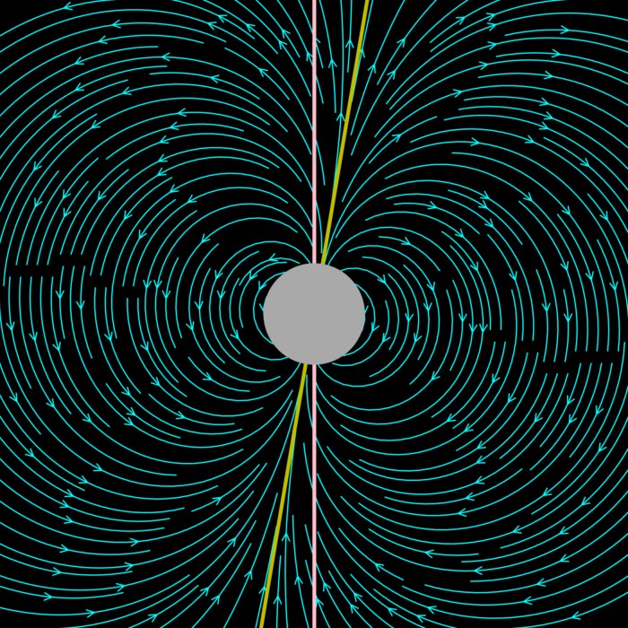
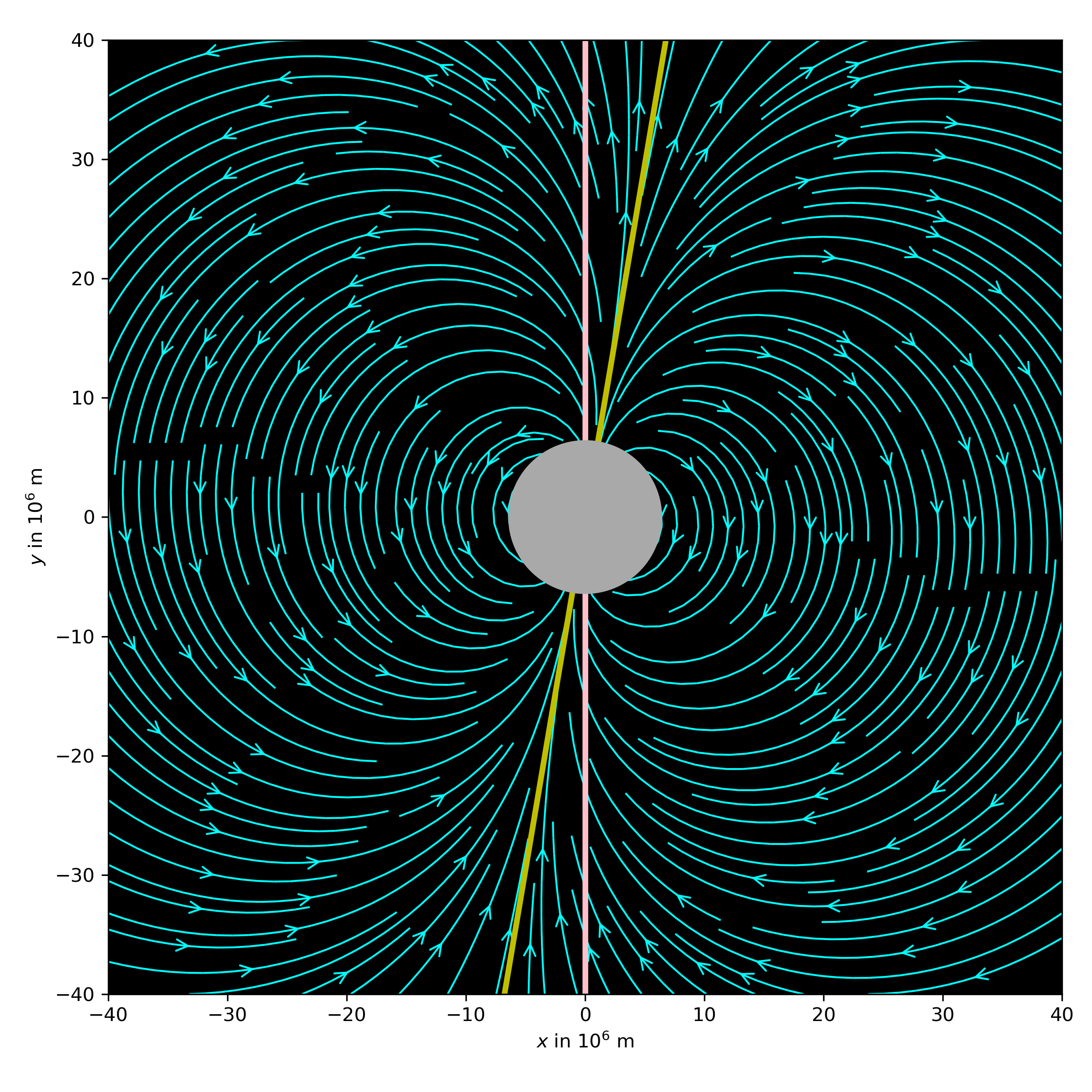Earth’s dipole magnetic field.

Conclusion

The code example demonstrates, that it takes not much to calculate and visualize complex physical phenomena using Python. The magnetic field of Earth is a fascinating topic, and I hope you enjoyed this post. If you have any questions or comments, please let me know in the comment below.

You can find the original code on scipython.comꜛ and the modified version in this GitHub repositoryꜛ.